Lug and Pin Analysis — Air Force Method (AFFDL-TR-69-42, Bruhn D1): Lug Bearing, Net Section, Transverse and Oblique Strength, Pin Shear and Bending, Press-Fit Bushings
Axial, transverse and oblique lug strength, pin shear and bending, bushing bearing, press-fit stresses and lug fatigue life, worked by the Air Force method of AFFDL-TR-69-42 (Bruhn D1). Every margin names the check that governs it, and the ƒ icons show the formula behind each result.
Advanced method options
Show detailed calculation steps
How the Method Works
This page follows the Air Force Method, set out in Section 9 of the Stress Analysis Manual of the Air Force Flight Dynamics Laboratory (AFFDL-TR-69-42). Bruhn Chapter D1 reproduces the same curves, so the two names describe one method. It is empirical: the interaction between bearing, shear-out and hoop tension is messy enough that the manual rolls it into coefficients read off test-derived charts rather than deriving each mode separately.
The five failure modes
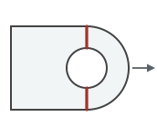
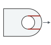
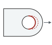
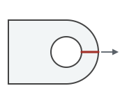
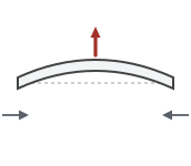
A pin-loaded lug can fail by tension across the net section, shear-out along two planes ahead of the hole, bearing against the pin, hoop tension across a single plane, or by buckling out of plane (“dishing”) if it is thin. The method folds the middle three — bearing, shear-out and hoop tension — into a single allowable, because in a real lug they are not independent.
Axial loading
The bearing allowable carries the combined bearing, shear-out and hoop tension behaviour in a single coefficient, read from Figure 9-2 as a function of e/D and D/t.
Net-section tension is checked separately, with the net-tension coefficient Kn from Figure 9-4 — a knockdown for the stress concentration at the hole that depends on the material's ultimate and yield strengths, modulus and ultimate strain.
In both, \( F_{u} \) is not simply Ftu: the manual caps the effective ultimate at \( \min\!\left(F_{tu},\; 1.304\,F_{ty}\right) \), which binds on materials with a high yield-to-ultimate ratio. That cap is applied here and shown in the calculation steps.
Single, double and multiple shear
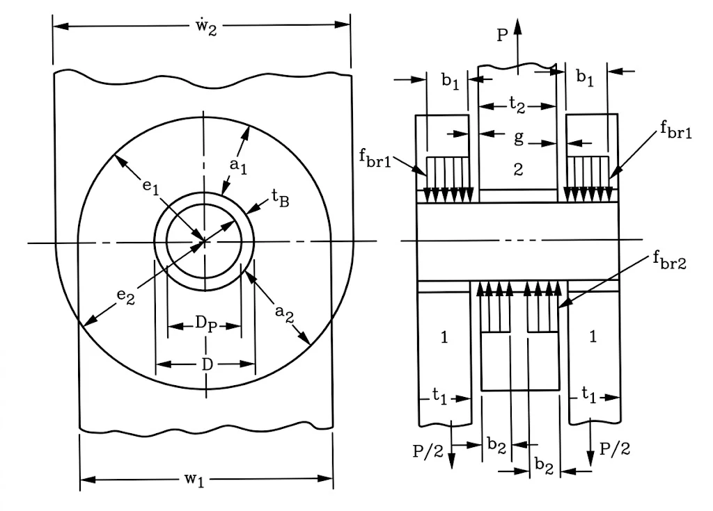
In a single-shear joint the two members are offset, so the load path is eccentric: the pin carries the whole load on one plane and the offset drives a bending moment through the joint. A double-shear (clevis) joint splits the load either side of the inner lug, halving the load on each pin plane and keeping the load path balanced. This is why the pin shear condition below changes the answer, and why the clevis gap sets the pin bending arm.

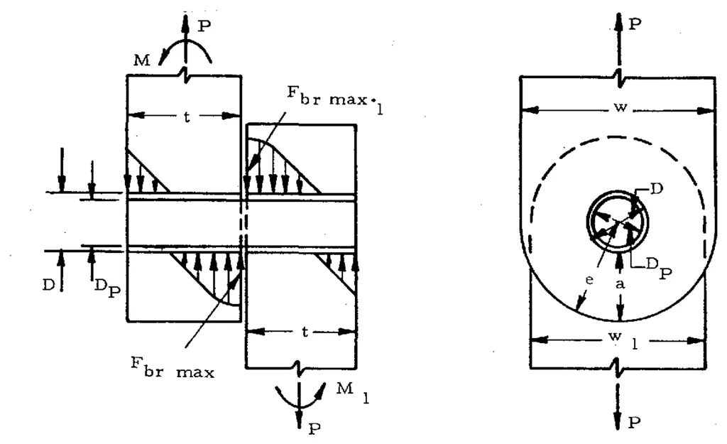
A hinge or a stacked fitting puts n lugs on one pin, interleaved from the two sides (Figure 9-13). The side with more lugs has (n + 1)/2 of them, the other (n − 1)/2. The manual (§9.13) does not ask for a pin-deflection analysis. It gives a load split (Table 9-2) that, at ultimate, leaves the pin almost straight. It assumes plastic lugs and an elastic pin.
- The inner lugs on the side with more lugs, all of thickness t′, carry P1 each.
- The two outermost lugs on that side carry only C P1. They may be as thin as C t′.
- Every lug on the other side, of thickness t″, carries P2 = P/[(n − 1)/2].
So P = P1[(n + 1)/2 − 2 + 2C]. The pin sees a peak shear ksP1 on one plane and a moment M = P1b/2:
| Lugs, both sides | C | Peak pin shear | b |
|---|---|---|---|
| 5 | 0.35 | 0.50 P1 | 0.28 (t′ + t″)/2 |
| 7 | 0.40 | 0.53 P1 | 0.33 (t′ + t″)/2 |
| 9 | 0.43 | 0.54 P1 | 0.37 (t′ + t″)/2 |
| 11 | 0.44 | 0.54 P1 | 0.39 (t′ + t″)/2 |
| ∞ (13 or more here) | 0.50 | 0.50 P1 | 0.50 (t′ + t″)/2 |
Choose Multiple under Pin shear condition, set the lug count, and enter t″ as the thickness and t′ as the other side’s inner lugs. The outermost lugs default to the minimum C t′. Each lug is then checked at its own load, with its own bearing coefficient: a thin outermost lug has a large D/t and can govern even though it carries least. The pin is checked against one shear plane, 0.785 D²Fsu, and against Mu = 0.0982 kbD³Ftu. The gap does not enter. Tangs are not checked in this mode.
Transverse loading
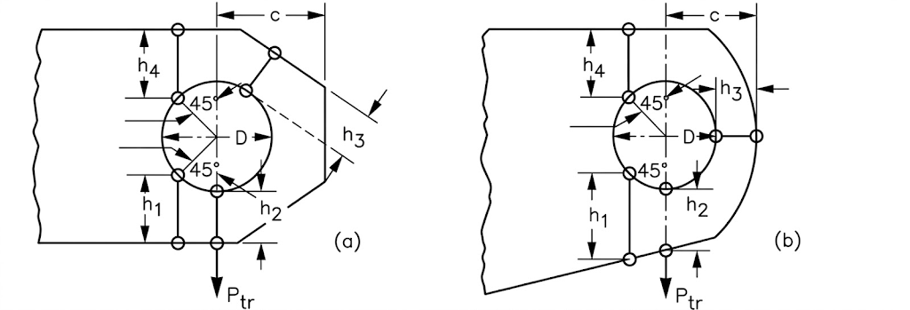
Loading a lug across its axis rather than along it engages a different, more redundant load path, so it gets its own coefficient family from Figure 9-8. That curve is driven by an effective edge distance hav, averaged from four radial distances between the hole and the lug boundary — which means a proper transverse check needs more of the lug outline than a single edge distance describes.
Oblique loading
A load at an angle is resolved into its axial and transverse components and recombined against the two pure allowables by a power-law interaction, with an exponent of 1.6:
\( \left(\dfrac{P_{ax}}{P_{u}}\right)^{1.6} + \left(\dfrac{P_{tr}}{P_{tru}}\right)^{1.6} = 1 \)
The exponent matters. A plain ellipse (exponent 2) reads about 9% high at 45°, in the unconservative direction. The “allowable vs load angle” chart above is this envelope, sliced along the applied angle.
What This Page Computes
Each lug — the inner lug and the outer lugs of a clevis, or the two lugs of a single-shear joint — is worked through the full method:
- Axial bearing — \( P_{bru} = K_{br}\,F_{u}\,D\,t \), with Kbr from Figure 9-2 at D/t ≤ 5 and Figure 9-3 above. This one coefficient covers bearing, shear-out and hoop tension together, so there is no separate tear-out check.
- Axial net section — \( P_{nu} = K_{n}\,F_{u}\,(W - D)\,t \), with Kn from Figure 9-4 at the material’s Fty/Ftu and Ftu/(Eεu).
- Transverse — \( P_{tru} = K_{tru}\,F_{tu}\,D\,t \) from Figure 9-8, at the effective edge distance hav of Figure 9-10.
- Oblique — the two combined by the 1.6-power interaction at the applied angle.
- Fatigue (optional) — life of a 2024-T3 or 7075-T6 lug under constant-amplitude axial load, §9.17, from Figures 9-23 to 9-26.
Fu = min(Ftu, 1.304 Fty) throughout. A bushing is checked at 1.304 Fcy on its bore. In double shear the joint allowable is equation 9-19: the lower of the inner lug-bushing strength and twice the outer, pin shear, and pin bending — with the balanced-design value of equation 9-16 when the pin is weak in bending. In single shear the lug moment amplifies the bearing and net-section stress (equations 9-23 to 9-27). Lugs under 5% elongation are reduced by the §9.15 ductility factor.
Reading a margin
MS = Pallow/P − 1. A margin at or above +0.15 shows as PASS, between 0 and +0.15 as MARGINAL, and below zero as FAIL. Those bands are a display convention on this page, not a certification requirement — the margin your programme demands is the one that governs.
Limitations
The coefficients are read off digitized charts and interpolated linearly between curves, so expect agreement with a careful hand reading to about the width of a pencil line — a percent or two. Outside a chart’s range the nearest edge is held and the calculation steps say so.
- The outer lugs (double shear) or mating lug (single shear) share the width, edge distance and material of the lug entered. A clevis with different outer-lug geometry needs a second run with those values.
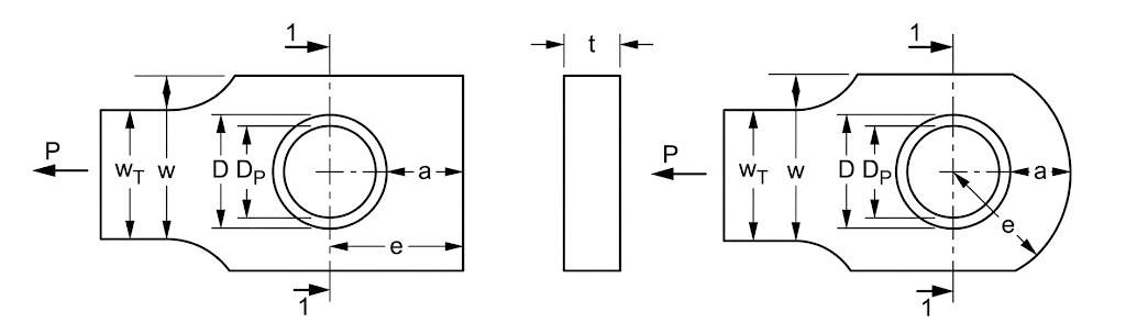
- Figure 9-10 assumes a concentric lug, whose head radius is both e and W/2; the smaller of the two is used. For any other outline, measure h1 to h4 as in Figure 9-7 and enter them under Advanced method options; the page then computes hav directly instead of reading the chart.
- In single shear the lug moment is split equally, M = P(t + t1)/4, which assumes neither member restrains the joint. Enter a moment from your own load path if the structure carries part of it.
- Kn uses the published elongation as the ultimate strain εu. Where none is published, the least ductile curve (Ftu/Eεu = 1.0) is used, which is conservative.
- Not checked: out-of-plane buckling of thin lugs and yield-load limits. Lug tangs (§9.4.4) are checked in double shear only, as the manual gives them. Fatigue (§9.17) covers constant-amplitude axial load on 2024-T3 and 7075-T6 lugs only; see Lug fatigue.
Materials
Properties come from the same MIL-HDBK-5 dataset behind the Material Property Lookup and Multi-Material Comparison, so Ftu, Fty, Fsu and Fbru are published allowables rather than typical values. The short list covers the common aerospace picks; ticking Full MIL-HDBK-5 database opens every published condition — alloy, product form, temper, thickness band and A/B/S basis — along with grain direction and a service temperature that derates the strengths off the effect-of-temperature curves.
Beyond the strengths, the method reads the modulus E and elongation (for Kn, the pin plastic bending coefficient and the §9.15 low-ductility check), Fcy for a bushing, and the e/D = 2.0 bearing allowables, which cap the lug bearing (Pbru/Dt may not exceed Fbru or 1.304 Fbry). A service temperature derates the yield-type values along with Fty. Every one of these is named in the calculation steps.
Interference-fit bushings
A bushing pressed into a lug with negative clearance squeezes the hole outward. Treating the lug head as a thick ring and the bushing as a thick tube, the contact pressure is set by the two radial displacements adding up to the interference (§9.16, equations 9-36 to 9-38):
\[ p = \frac{\delta}{\dfrac{D}{E_{ring}}\left(\dfrac{C^2+D^2}{C^2-D^2}+\mu_{ring}\right) + \dfrac{B}{E_{bush}}\left(\dfrac{B^2+A^2}{B^2-A^2}-\mu_{bush}\right)} \]with A the bushing bore radius, B its outside radius, C the lug outer radius and D the hole radius; δ is the radial interference, half the diametral interference entered above. The hole sees a hoop tension \( F_t = p\,(C^2+D^2)/(C^2-D^2) \) and the bushing bore a hoop compression \( 2pB^2/(B^2-A^2) \).
The manual limits the sustained hoop stress rather than letting it run to yield: 0.50 Fty for aluminum alloys and 8,000 psi for magnesium (stress corrosion), and 25% of Ftu for steel heat treated above 200 ksi (hydrogen embrittlement). The bushing bore is checked against its compressive yield. A moderate press fit helps fatigue, because the hoop preload cuts the stress range under oscillating loads.
Lug fatigue
Section 9.17 of the manual predicts the fatigue life of 2024-T3 and 7075-T6 aluminum lugs under constant-amplitude axial load. It is an empirical fit to lug tests, not a stress-concentration calculation. Three factors from Figure 9-23 describe how severe a lug is, and their product k1k2k3 picks one curve from a family of R = 0 life curves (Figure 9-24 for 7075-T6, 9-25 for 2024-T3). A higher product is a better lug and sits on a higher curve.
- k1 is read against a/C, where a is the end distance from the edge of the hole to the end of the lug and C the side distance from the edge of the hole to the side (Figure 9-21). For the lug drawn here, a = e − D/2 and C = (W − D)/2.
- k2 is read against D/C.
- k3 is read against the hole diameter D in inches: a size effect.
For 2024-T3 a single line serves for both k1 and k2. The method is only claimed inside the shaded region of Figure 9-22: C/D from 0.3 to 2.0 and a/C from 0.8 to 2.0, with the corner cut at a/C + C/D = 3.5. Outside it the manual asks for tests, and the page says so.
The printed curves stop at a few hundred to a thousand cycles. To reach static failure, the manual replaces the top of the chosen curve with a straight line on the semi-log axes. The line runs from 0.5 Fnu at one cycle down to where the curve crosses 0.4 Fnu. Here Fnu is the net-tension ultimate stress of §9.3.2, KnFu. At R = 0, 0.4 Fnu is the alternating stress whose peak is 0.8 Fnu, the manual’s average yield for these alloys.
The mean stress is then handled with a Goodman diagram (Figure 9-26). Each constant-life line runs from the R = 0 point (fa0, fa0) to (Fnu, 0). Instead of drawing the diagram, the page solves that line for the R = 0 amplitude equivalent to the applied cycle, then reads its life off the curve:
\[ f_a = \frac{f_{max}-f_{min}}{2},\qquad f_m = \frac{f_{max}+f_{min}}{2},\qquad f_{a0} = \frac{f_a\,F_{nu}}{F_{nu}-f_m+f_a} \]When a required life is entered, the curve gives fa0 at that life. The same Goodman line then gives the largest peak stress allowed at the applied stress ratio R = fmin/fmax:
\[ f_{max,allow} = \frac{f_{a0}\,F_{nu}}{(1-R)\,F_{nu}/2 + R\,f_{a0}} \]The tile’s margin is fmax,allow/fmax − 1, a margin on stress, not on life. All stresses are net-section stresses on the inner lug, P/((W − D)t), with the hole diameter taken as the bushing OD when a bushing is fitted.
Check against the manual (§9.18). The example is a concentric 7075-T6 lug with a = C = 0.344 in and D = 0.437 in.
- Figure 9-23 gives k1 = 1.0, k2 = 1.33 and k3 = 0.99. The digitized charts give 1.008, 1.322 and 0.996.
- With Fnu = 70 ksi and a cycle of 27,700/18,470 psi, the manual reads N = 8×10⁴ from its Goodman diagram. The test result was 8.6×10⁴. The same inputs here give 7.7×10⁴.
- The manual’s table of fa against N for this lug is matched to within 0.3 ksi at every life except 104 cycles (12.7 against 13.5 ksi). That is the tolerance of reading the scan.
Limits. Constant-amplitude, axial loading only: no spectrum, no transverse or oblique fatigue load, no fretting allowance. A compressive minimum load extrapolates the Goodman line below R = 0, where the tests did not go. The single-shear bending moment is not included. Any other alloy is read on the curve family chosen, and the page flags that as an estimate. A press fit generally improves fatigue life, but this method does not credit it.
Verification
The calculation engine (js/lug-math.js) is run in automated
tests against the worked example in §9.6 of the manual, the NASA
reproduction of Bruhn’s peaking-factor chart, and hand calculations
of the press-fit equations.
| Case | Reference | This page | Note |
|---|---|---|---|
| §9.6 female lug bearing Pbru | 28,600 lb | 28,451 lb | K read off Fig. 9-2 |
| §9.6 female lug Kn | 0.74 | 0.738 | |
| §9.6 male lug bearing Pbru | 77,000 lb | 77,374 lb | |
| §9.6 male lug Kn | 0.87 | 0.873 | The manual then uses 1.304 Fty, although Ftu < 1.304 Fty and eq. 9-6a applies. Bearing governs either way. |
| §9.6 pin bending Pubp | 30,100 lb | 30,044 lb | eq. 9-15 |
| §9.6 balanced design = joint allowable | 37,900 lb | 37,805 lb | eq. 9-16; b1, 2b2 = 0.332, 0.644 in (manual 0.331, 0.646) |
| Peaking factor γ at q = 1.0, r = 0.1 / 0.2 / 0.3 | 0.905 / 0.82 / 0.725 | 0.905 / 0.820 / 0.726 | Read off NASA TM X-73305 Fig. B 2.1.0-6 |
| Press-fit pressure p (A 0.5, B 1.00025, C 1.5, D 0.9975 in; steel bushing in aluminum) | 8,600.16 psi | 8,600.16 psi | Eq. 9-36 to 9-38 by hand; lug hoop 22,237 psi |
The peaking factor γ of the Bruhn pin-bending option is Bruhn’s Fig. D1.15 as reproduced in the NASA Astronautic Structures Manual, traced from the NASA scan. Its dashed starting portions are, in the manual’s words, not substantiated by test data.
Worked Example: The Manual’s Double-Shear Joint
Section 9.6 of AFFDL-TR-69-42 works a complete double-shear joint by hand. It is worth following once, because every step on this page is one of these steps. The two outer (female) lugs are 2024-T351 plate, the inner (male) lug 7075-T651, each with an aluminum-bronze bushing on a 3/4″ 4130 steel pin; the gap between lugs is g = 0.10″. The page reproduces the manual’s numbers in its automated tests; they are shown below side by side.
| Outer (female) lugs | Inner (male) lug | Bushings | Pin | |
|---|---|---|---|---|
| Material | 2024-T351 plate | 7075-T651 plate | Al bronze | 4130 steel |
| Ftu / Fty | 64 / 40 ksi | 77 / 66 ksi | Fcy 60 ksi | 125 ksi, Fsu 82 ksi |
| E, εu | 10.5 Msi, 0.12 | 10.3 Msi, 0.06 | kb = 1.56 | |
| D, e, w, t | 1.00, 1.25, 2.50, 0.50 in | 1.00, 1.50, 3.00, 0.75 in | Dp = 0.75 in | Dp = 0.75 in |
| Quantity | Manual | This page |
|---|---|---|
| Outer lug Pbru / Kn | 28,600 lb / 0.74 | 28,451 lb / 0.738 |
| Inner lug Pbru / Kn | 77,000 lb / 0.87 | 77,374 lb / 0.873 |
| Pin bending Pubp | 30,100 lb | 30,044 lb |
| Balanced design = joint allowable | 37,900 lb | 37,805 lb |
| Effective widths b1, 2b2 | 0.331, 0.646 in | 0.332, 0.644 in |
The pin governs, and it does so by bending, not shear: at 37,900 lb the joint is worth only 86% of the lug-bushing strength. The balanced-design widths say the same thing from the other side: lugs thicker than b1 = 0.33″ and 2b2 = 0.65″ carry no extra load with this pin, so a lighter design would thin the lugs or a stronger one would enlarge the pin. The manual prints the inner lug’s net section as 112,313 lb using 1.304 Fty, but Ftu < 1.304 Fty for this 7075, so equation 9-6a (KnFtu) applies; bearing governs that lug either way.
This joint cannot be loaded straight into the calculator: the page uses one material and one lug outline for the inner and outer lugs, and its materials come from MIL-HDBK-5 design allowables rather than the manual’s Table 9-1. Running the inner lug as entered and the outer lug as a second run with its own geometry reproduces the same steps.
References
- Air Force Flight Dynamics Laboratory (1986). Stress Analysis Manual, AFFDL-TR-69-42, Section 9, Lug Analysis. Open Section 9.
- Melcon, M. A. and Hoblit, F. M. (1953). “Developments in the analysis of lugs and shear pins.” Product Engineering, 24(6), 160–170. The source of the Air Force method’s coefficient charts.
- Cozzone, F. P., Melcon, M. A. and Hoblit, F. M. (1950). “Analysis of lugs and shear pins made of aluminum or steel alloys.” Product Engineering, 21(5), 113–117.
- Bruhn, E. F. (1973). Analysis and Design of Flight Vehicle Structures. Jacobs Publishing. Chapter D1, lugs and shear pins, including the pin-bending peaking factor.
- NASA (1975). Astronautic Structures Manual, NASA TM X-73305, Volume I, Section B2, Lugs and Shear Pins. Open Section B2 (PDF, 27.8 MB). Volumes II and III cover stability, thermal stress and composites.
- Department of Defense (2003). MIL-HDBK-5J, Metallic Materials and Elements for Aerospace Vehicle Structures. The design allowables used here.
- ESDU 91008 (1991). Design against fatigue: lugs, and related ESDU static-strength data items. A widely used alternative to the Air Force method.
The coefficient charts the Air Force method is built on, digitized point-for-point from the scanned plots and redrawn here so a value can be read off a curve rather than interpolated by eye. Hover any curve for a readout; each series is densified to a fine grid, so the tooltip tracks the line continuously instead of snapping between digitized vertices.
These are the calculator’s inputs. The same arrays drive the margins above, so a value hovered here is the value the calculation reads.
Figure 9-2. Allowable uniform axial load coefficient. Valid for D/t ≤ 5, which covers most lugs. The curve is one line; it is split here because the formula it feeds changes at e/D = 1.5 — below that the allowable is \( K\,a\,t\,F_{tux} \) using the nose distance a, above it \( K\,D\,t\,F_{tux} \) using the hole diameter. The minimum of 1.33 sits exactly at the changeover.
Figure 9-3. Bearing efficiency factors, used in place of Figure 9-2 once D/t exceeds 5. The scan labels the abscissa a/D, but every curve reaches zero at 0.5, where the hole breaks out of the edge — that is e/D = 0.5, and Bruhn D1.12 plots the same curves against e/D. It is redrawn here on e/D. The dashed cutoffs cap K for aluminium: (A) for hand forged billet with the long transverse grain across the lug, (B) for plate, bar and hand forged billet with the short transverse grain across it. The original also caps K at 2.00 for lugs cut from aluminium 0.5″ or thicker. The chart is drawn for aluminium alloys and alloy steel below 160 ksi.
Figure 9-4(b). Net-tension stress coefficient for Fty/Ftu = 1.0. The net-section allowable is \( K_{n}\,F_{tu}\,(w - D)\,t \). Kn is a knockdown for the stress concentration at the hole, relieved by the material's ability to yield — which is why the curve family is indexed on Ftu/(E·εu), a measure of how brittle the material is.
Figure 9-4(c). Net-tension stress coefficient for Fty/Ftu = 0.8. Interpolate between panels on the yield-to-ultimate ratio; most structural alloys land between this panel and (b).
Figure 9-4(d). Net-tension stress coefficient for Fty/Ftu = 0.6. The lowest ratio the manual plots; below it the curves are extrapolated rather than read.
Figure 9-8. Transverse ultimate and yield load coefficients against the effective edge distance hav/D. The two curves run together to about hav/D = 0.8 and then separate, Ktru above Ktry. The transverse allowable is \( K_{tru}\,F_{tux}\,D\,t \); there is no separate transverse net-section check in the method.
Figure 9-10. Effective edge distance for a concentric lug with parallel sides — the geometry this calculator draws. For that shape hav/D reads straight off e/D, which sidesteps measuring the four radial distances h1–h4 of Figure 9-7 and working the nomograph of Figure 9-9. For any other outline, enter the four distances under Advanced method options and the page computes hav = 6/(3/h1 + 1/h2 + 1/h3 + 1/h4), the relation the nomograph of Figure 9-9 solves graphically.
Figure 9-17. Ductility factor for lugs whose material has less than 5% elongation (§9.15). B is read twice at the same Fty/Ftu: once at the material’s own εy/εu and once as if εu were 0.05. The bearing and transverse allowables are multiplied by the ratio B/B.05. The curves fall to a common floor of B = 0.663. Traced from a 400 dpi render of the scan, with each point snapped to the centre of the printed line.
Pin-bending peaking factor γ (Bruhn Fig. D1.15), used by the Bruhn pin-bending option. The pin-bending arm is t1/2 + g + γt2/4. The x-axis is the inner lug’s strength ratio (P′u)min/(AbrFtux), and the curves are r = (e/D − 0.5)D/t2. Each curve starts on the line γ = 0.5×ratio, drawn dashed, and nothing reads below it. Traced from the NASA Astronautic Structures Manual reproduction of the chart (Fig. B 2.1.0-6), each curve followed on the ink of a 400 dpi render.
Figure 9-23. The three lug fatigue parameters of §9.17. k1 is read against a/C (end distance over side distance, both from the edge of the hole), k2 against D/C and k3 against the hole diameter D in inches. For 2024-T3 one line serves for both k1 and k2. Their product picks the curve on Figure 9-24 or 9-25. Traced from a 400 dpi render, with each point snapped to the printed line.
Figure 9-24. Fatigue curves for 7075-T6 lugs at R = 0: the alternating net-section stress fa at failure against life, one curve per k1k2k3. The calculator interpolates linearly between curves and replaces the low-cycle end with the straight line of step 4, from 0.5 Fnu at one cycle to where the curve crosses 0.4 Fnu. The trace reproduces the manual’s own table for k1k2k3 = 1.32 to within 0.3 ksi, except at 104 cycles (12.7 against 13.5 ksi).
Figure 9-25. The same family for 2024-T3 lugs. The upper five curves start at 103 cycles and the lower five earlier; all ten flatten together past 106. Below k1k2k3 = 0.8, past 2×10⁶ cycles, the printed curves run into the axis and the trace is less certain.