Since many aerospace companies manufacture both commercial and military products, the standardization of metallic materials design data, which are acceptable to Government procuring or certification agencies is very beneficial to those manufacturers as well as governmental agencies. Although the design requirements for military and commercial products may differ greatly, the required design values for the strength of materials and elements and other needed material characteristics are often identical. Therefore, this publication provides standardized design values and related design information for metallic materials and structural elements used in aerospace structures. The data contained herein, or from approved items in the minutes of MIL-HDBK-5 coordination meetings, are acceptable to the Air Force, the Navy, the Army, and the Federal Aviation Administration. Approval by the procuring or certificating agency must be obtained for the use of design values for products not contained herein.
This printed document is distributed by the Document Automation and Production Service (DAPS). It is the only official form of MIL-HDBK-5. If computerized third-party MIL-HDBK-5 databases are used, caution should be exercised to ensure that the information in these databases is identical to that contained in this Handbook.
U.S. Government personnel may obtain free copies of the current version of the printed document from the Document Automation and Production Service (DAPS). Assistance with orders may be obtained by calling (215) 697-2179. The FAX number is (215) 697-1462. U.S. Government personnel may also obtain a free electronic copy of the current document from DAPS through the ASSIST website at http://assist.daps.mil.
This Handbook is primarily intended to provide a source of design mechanical and physical properties, and joint allowables. Material property and joint data obtained from tests by material and fastener producers, government agencies, and members of the airframe industry are submitted to MIL-HDBK-5 for review and analysis. Results of these analyses are submitted to the membership during semi-annual coordination meetings for approval and, when approved, published in this Handbook.
This Handbook also contains some useful basic formulas for structural element analysis. However, structural design and analysis are beyond the scope of this Handbook.
References for data and various test methods are listed at the end of each chapter. The reference number corresponds to the applicable paragraph of the chapter cited. Such references are intended to provide sources of additional information, but should not necessarily be considered as containing data suitable for design purposes.
The content of this Handbook is arranged as follows:
- Chapter 1 — Nomenclature, Systems of Units, Formulas, Material Property Definitions, Failure Analysis, Column Analysis, Thin-Walled Sections
- Chapters 2 — Steel Properties
- Chapters 3 — Aluminum Properties
- Chapters 4 — Magnesium Properties
- Chapters 5 — Titanium Properties
- Chapters 6 — Cobalt Base Alloys Properties
- Chapters 7 — Misc Alloys and Hybrid Material Properties
- Chapter 8 — Joint Allowables
- Chapter 9 — Data Requirements, Statistical Analysis Procedures
The various symbols used throughout the Handbook to describe properties of materials, grain directions, test conditions, dimensions, and statistical analysis terminology are included in Appendix A.
Design properties and joint allowables contained in this Handbook are given in customary units of U.S. measure to ensure compatibility with government and industry material specifications and current aerospace design practice. Appendix A.4 may be used to assist in the conversion of these units to Standard International (SI) units when desired.
Formulas provided in the following sections are listed for reference purposes. Sign conventions generally accepted in their use are that quantities associated with tension action (loads, stresses, strains, etc.) are usually considered as positive and quantities associated with compressive action are considered as negative. When compressive action is of primary interest, it is sometimes convenient to identify associated properties with a positive sign. Formulas for all statistical computations relating to allowables development are presented in Chapter 9.
tubes due to torsion
in thin-walled structures of closed section.
Note that A is the area enclosed
by the median line of the section.
stresses, where B = biaxial ratio
obtained from the same tests in
which f and e are measured.
when the deflection is to be calculated
using a known value of E.)
radians per unit length
(This integral denotes the area under
the curve of M/EI plotted against x,
between the limits of x1 and x2.)
(This integral denotes the area under the curve having an ordinate equal to M/EI multiplied by the corresponding distances to Point 2, plotted against x, between the limits of x1 and x2.)
(This integral denotes the area under
the curve of x1(i) plotted against x,
between the limits of x1 and x2.)
or twist per unit length of
a member,radians per unit length.)
(This integral denotes the area under
the curve of T/GJ plotted against x,
between the limits of x1 and x2.)
is constant over length L.
deformation.) This identifies Poisson’s
ratio in uniaxial loading.
inelastic or plastic strain response
where
Equation 1.3.9(b) implies a log-linear relationship between inelastic strain and stress, which is observed with many metallic materials, at least for inelastic strains ranging from the material's proportional limit to its yield stress.
It is assumed that users of this Handbook are familiar with the principles of strength of materials. A brief summary of that subject is presented in the following paragraphs to emphasize principles of importance regarding the use of allowables for various metallic materials.
Requirements for adequate test data have been established to ensure a high degree of reliability for allowables published in this Handbook. Statistical analysis methods, provided in Chapter 9, are standardized and approved by all government regulatory agencies as well as MIL-HDBK-5 members from industry.
Primary static design properties are provided for the following conditions:
- Tension — Ftu and Fty
- Compression — Fcy
- Shear — Fsu
- Bearing — Fbru and Fbry
These design properties are presented as A- and B- or S-basis room temperature values for each alloy. Design properties for other temperatures, when determined in accordance with Section 1.4.1.3, are regarded as having the same basis as the corresponding room temperature values.
Elongation and reduction of area design properties listed in room temperature property tables represent procurement specification minimum requirements, and are designated as S-values. Elongation and reduction of area at other temperatures, as well as moduli, physical properties, creep properties, fatigue properties and fracture toughness properties are all typical values unless another basis is specifically indicated.
Use of B-Values — The use of B-basis design properties is permitted in design by the Air Force, the Army, the Navy, and the Federal Aviation Administration, subject to certain limitations specified by each agency. Reference should be made to specific requirements of the applicable agency before using B-values in design.
Statistically calculated values are S (since 1975), T99 and T90. S, the minimum properties guaranteed in the material specification, are calculated using the same requirements and procedure as AMS and is explained in Chapter 9. T99 and T90 are the local tolerance bounds, and are defined and may be computed using the data requirements and statistical procedures explained in Chapter 9.
A ratioed design property is one that is determined through its relationship with an established design value. This may be a tensile stress in a different grain direction from the established design property grain direction, or it may be another stress property, e.g., compression, shear or bearing. It may also be the same stress property at a different temperature. Refer to Chapter 9 for specific data requirements and data analysis procedures.
Derived properties are presented in two manners. Room temperature derived properties are presented in tabular form with their baseline design properties. Other than room temperature derived properties are presented in graphical form as percentages of the room temperature value. Percentage values apply to all forms and thicknesses shown in the room temperature design property table for the heat
treatment condition indicated therein unless restrictions are otherwise indicated. Percentage curves usually
represent short time exposures to temperature (thirty minutes) followed by testing at the same strain rate
as used for the room temperature tests. When data are adequate, percentage curves are shown for other
exposure times and are appropriately labeled.
The term "stress" as used in this Handbook implies a force per unit area and is a measure of the intensity of the force acting on a definite plane passing through a given point (see Equations 1.3.2(a) and 1.3.2(b)). The stress distribution may or may not be uniform, depending on the nature of the loading condition. For example, tensile stresses identified by Equation 1.3.2(a) are considered to be uniform. The bending stress determined from Equation 1.3.2(c) refers to the stress at a specified distance perpendicular to the normal axis. The shear stress acting over the cross section of a member subjected to bending is not uniform. (Equation 1.3.2(d) gives the average shear stress.)
Strain is the change in length per unit length in a member or portion of a member. As in the case of stress, the strain distribution may or may not be uniform in a complex structural element, depending on the nature of the loading condition. Strains usually are present also in directions other than the directions of applied loads.
A normal strain is that which is associated with a normal stress; a normal strain occurs in the direction in which its associated normal stress acts. Normal strains that result from an increase in length are designated as positive (+) and those that result in a decrease in length are designated as negative (−).
Under the condition of uniaxial loading, strain varies directly with stress. The ratio of stress to strain has a constant value (E) within the elastic range of the material, but decreases when the proportional limit is exceeded (plastic range). Axial strain is always accompanied by lateral strains of opposite sign in the two directions mutually perpendicular to the axial strain. Under these conditions, the absolute value of a ratio of lateral strain to axial strain is defined as Poisson's ratio. For stresses within the elastic range, this ratio is approximately constant. For stresses exceeding the proportional limit, this ratio is a function of the axial strain and is then referred to as the lateral contraction ratio. Information on the variation of
Poisson’s ratio with strain and with testing direction is available in Reference 1.4.3.1.
Under multiaxial loading conditions, strains resulting from the application of each directional load are additive. trains must be calculated for each of the principal directions taking into account each of the principal stresses and Poisson’s ratio (see Equation 1.3.7 for biaxial loading).
When an element of uniform thickness is subjected to pure shear, each side of the element will be displaced in opposite directions. Shear strain is computed by dividing this total displacement by the right angle distance separating the two sides.
Strain rate is a function of loading rate. Test results are dependent upon strain rate, and the ASTM testing procedures specify appropriate strain rates. Design properties in this Handbook were developed from test data obtained from coupons tested at the stated strain rate or up to a value of 0.01 in./in./min, the standard maximum static rate for tensile testing materials per specification ASTM E 8.
Elongation and reduction of area are measured in accordance with specification ASTM E 8.
When a metallic specimen is tested in tension using standard procedures of ASTM E 8, it is customary to plot results as a "stress-strain diagram." Typical tensile stress-strain diagrams are characterized in Figure 1.4.4. Such diagrams, drawn to scale, are provided in appropriate chapters of this Handbook. The general format of such diagrams is to provide a strain scale nondimensionally (in./in.) and a stress scale in 1000 lb/in.² (ksi). Properties required for design and structural analysis are discussed in Sections 1.4.4.1 to 1.4.4.6.
Referring to Figure 1.4.4, it is noted that the initial part of stress-strain curves are straight lines. This indicates a constant ratio between stress and strain. Numerical values of such ratios are defined as the modulus of elasticity, and denoted by the letter E. This value applies up to the proportional limit stress at which point the initial slope of the stress-strain curve then decreases. Modulus of elasticity has the same units as stress. See Equation 1.3.4(b).
Other moduli of design importance are tangent modulus, Et, and secant modulus, Es. Both of these moduli are functions of strain. Tangent modulus is the instantaneous slope of the stress-strain curve at any elected value of strain. Secant modulus is defined as the ratio of total stress to total strain at any selected value of strain. Both of these moduli are used in structural element designs. Except for materials such as those described with discontinuous behaviors, such as the upper stress-strain curve in Figure 1.4.4, tangent modulus is the lowest value of modulus at any state of strain beyond the proportional limit. Similarly, secant modulus is the highest value of modulus beyond the proportional limit.
Clad aluminum alloys may have two separate modulus of elasticity values, as indicated in the typical stress-strain curve shown in Figure 1.4.4. The initial slope, or primary modulus, denotes a response of both the low-strength cladding and higher-strength core elastic behaviors. This value applies only up to the proportional limit of the cladding. For example, the primary modulus of 2024-T3 clad sheet applies only up to about 6 ksi. Similarly, the primary modulus of 7075-T6 clad sheet applies only up to approximately 12 ksi. A typical use of primary moduli is for low amplitude, high frequency fatigue. Primary moduli are not applicable at higher stress levels. Above the proportional limits of cladding materials, a short transition range occurs while the cladding is developing plastic behavior. The material then exhibits a secondary elastic modulus up to the proportional limit of the core material. This secondary modulus is the slope of the second straight line portion of the stress-strain curve. In some cases, the cladding is so little different from the core material that a single elastic modulus value is used.
The tensile proportional limit is the maximum stress for which strain remains proportional to stress. Since it is practically impossible to determine precisely this point on a stress-strain curve, it is customary to assign a small value of plastic strain to identify the corresponding stress as the proportional limit. In this Handbook, the tension and compression proportional limit stress corresponds to a plastic strain of 0.0001 in./in.
Stress-strain diagrams for some ferrous alloys exhibit a sharp break at a stress below the tensile ultimate strength. At this critical stress, the material elongates considerably with no apparent change in stress. See the upper stress-strain curve in Figure 1.4.4. The stress at which this occurs is referred to as the yield point. Most nonferrous metallic alloys and most high strength steels do not exhibit this sharp break, but yield in a monotonic manner. Permanent deformation may be detrimental, and the industry adopted 0.002 in./in. plastic strain as an arbitrary limit that is considered acceptable by all regulatory agencies. For tension and compression, the corresponding stress at this offset strain is defined as the yield stress (see Figure 1.4.4). This value of plastic axial strain is 0.002 in./in. and the corresponding stress is defined as the yield stress. For practical purposes, yield stress can be determined from a stress-strain diagram by extending a line parallel to the elastic modulus line and offset from the origin by an amount of 0.002 in./in. strain. The yield stress is determined as the intersection of the offset line with the stress-strain curve.
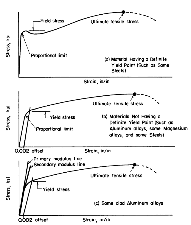
Figure 1.4.4 shows how the tensile ultimate stress is determined from a stress-strain diagram. It is simply the maximum stress attained. It should be noted that all stresses are based on the original cross-sectional dimensions of a test specimen, without regard to the lateral contraction due to Poisson's ratio effects. That is, all strains used herein are termed engineering strains as opposed to true strains which take into account actual cross sectional dimensions. Ultimate tensile stress is commonly used as a criterion of the strength of the material for structural design, but it should be recognized that other strength properties may often be more important.
An additional property that is determined from tensile tests is elongation. This is a measure of ductility. Elongation, also stated as total elongation, is defined as the permanent increase in gage length, measured after fracture of a tensile specimen. It is commonly expressed as a percentage of the original gage length. Elongation is usually measured over a gage length of 2 inches for rectangular tensile test specimens and in 4D (inches) for round test specimens. Welded test specimens are exceptions. Refer to the applicable material specification for applicable specified gage lengths. Although elongation is widely used as an indicator of ductility, this property can be significantly affected by testing variables, such as thickness, strain rate, and gage length of test specimens. See Section 1.4.1.1 for data basis.
Another property determined from tensile tests is reduction of area, which is also a measure of ductility. Reduction of area is the difference, expressed as a percentage of the original cross sectional area, between the original cross section and the minimum cross sectional area adjacent to the fracture zone of a tested specimen. This property is less affected by testing variables than elongation, but is more difficult to compute on thin section test specimens. See Section 1.4.1.1 for data basis.
Results of compression tests completed in accordance with ASTM E 9 are plotted as stress-strain curves similar to those shown for tension in Figure 1.4.4. Preceding remarks concerning tensile properties of materials, except for ultimate stress and elongation, also apply to compressive properties. Moduli are slightly greater in compression for most of the commonly used structural metallic alloys. Special considerations concerning the ultimate compressive stress are described in the following section. An evaluation of techniques for obtaining compressive strength properties of thin sheet materials is outlined in Reference 1.4.5
Since the actual failure mode for the highest tension and compression stress is shear, the maximum compression stress is limited to Ftu. The driver for all the analysis of all structure loaded in compression is the slope of the compression stress strain curve, the tangent modulus.
Compressive yield stress is measured in a manner identical to that done for tensile yield strength. It is defined as the stress corresponding to 0.002 in./in. plastic strain.
Results of torsion tests on round tubes or round solid sections are plotted as torsion stress-strain diagrams. The shear modulus of elasticity is considered a basic shear property. The theoretical ratio between shear and tensile stress for homogeneous, isotropic materials is 0.577. Reference 1.4.6 contains additional information on this subject.
This property is the initial slope of the shear stress-strain curve. It is also referred to as the modulus of elasticity in shear. The relation between this property and the modulus of elasticity in tension is expressed for homogeneous isotropic materials by the following equation:
This property is of particular interest in connection with formulas which are based on considerations of linear elasticity, as it represents the limiting value of shear stress for which such formulas are applicable. This property cannot be determined directly from torsion tests.
These properties, as usually obtained from ASTM test procedures tests, are not strictly basic properties, as they will depend on the shape of the test specimen. In such cases, they should be treated as moduli and should not be combined with the same properties obtained from other specimen configuration tests.
Design values reported for shear ultimate stress (Fsu) in room temperature property tables for aluminum and magnesium thin sheet alloys are based on “punch” shear type tests except when noted. Heavy section test data are based on “pin” tests. Thin aluminum products may be tested to ASTM B 831, which is a slotted shear test. Thicker aluminums use ASTM B 769, otherwise known as the Amsler shear test. These two tests only provide ultimate strength. Shear data for other alloys are obtained from pin tests, except where product thicknesses are insufficient. These tests are used for other alloys; however, the standards don’t specifically cover materials other than aluminum.
Bearing stress limits are of value in the design of mechanically fastened joints and lugs. Only yield and ultimate stresses are obtained from bearing tests. Bearing stress is computed from test data by dividing the load applied to the pin, which bears against the edge of the hole, by the bearing area. Bearing area is the product of the pin diameter and the sheet or plate thickness.
A bearing test requires the use of special cleaning procedures as specified in ASTM E 238. Results are identified as “dry-pin” values. The same tests performed without application of ASTM E 238 cleaning procedures are referred to as “wet pin” tests. Results from such tests can show bearing stresses at least 10 percent lower than those obtained from “dry pin” tests. See Reference 1.4.7 for additional information. Additionally, ASTM E 238 requires the use of hardened pins that have diameters within 0.001 of the hole diameter. As the clearance increases to 0.001 and greater, the bearing yield and failure stress tends to decrease.
In the definition of bearing values, t is sheet or plate thickness, D is the pin diameter, and e is the edge distance measured from the center of the hole to the adjacent edge of the material being tested in the direction of applied load.
BUS is the maximum stress withstood by a bearing specimen. BYS is computed from a bearing stress-deformation curve by drawing a line parallel to the initial slope at an offset of 0.02 times the pin diameter.
Tabulated design properties for bearing yield stress (Fbry) and bearing ultimate stress (Fbru) are provided throughout the Handbook for edge margins of e/D = 1.5 and 2.0. Bearing values for e/D of 1.5 are not intended for designs of e/D < 1.5. Bearing values for e/D < 1.5 must be substantiated by adequate tests, subject to the approval of the procuring or certificating regulatory agency. For edge margins between 1.5 and 2.0, linear interpolation of properties may be used.
Bearing design properties are applicable to t/D ratios from 0.25 to 0.50. Bearing design values for conditions of t/D < 0.25 or t/D > 0.50 must be substantiated by tests. The percentage curves showing temperature effects on bearing stress may be used with both e/D properties of 1.5 and 2.0.
Due to differences in results obtained between dry-pin and wet-pin tests, designers are encouraged to consider the use of a reduction factor with published bearing stresses for use in design.
Temperature effects require additional considerations for static, fatigue and fracture toughness properties. In addition, this subject introduces concerns for time-dependent creep properties.
Temperatures below room temperature generally cause an increase in strength properties of metallic alloys. Ductility, fracture toughness, and elongation usually decrease.
Temperatures above room temperature usually cause a decrease in the strength properties of metallic alloys. This decrease is dependent on many factors, such as temperature and the time of exposure which may degrade the heat treatment condition, or cause a metallurgical change. Ductility may increase or decrease with increasing temperature depending on the same variables. Because of this dependence of strength and ductility at elevated temperatures on many variables, it is emphasized that the elevated temperature properties obtained from this Handbook be applied for only those conditions of exposure stated herein.
The effect of temperature on static mechanical properties is shown by a series of graphs of property (as percentages of the room temperature allowable property) versus temperature. Data used to construct these graphs were obtained from tests conducted over a limited range of strain rates. Caution should be exercised in using these static property curves at very high temperatures, particularly if the strain rate intended in design is much less than that stated with the graphs. The reason for this concern is that at very low strain rates or under sustained loads, plastic deformation or creep deformation may occur to the detriment of the intended structural use.
Creep is defined as a time-dependent deformation of a material while under an applied load. It is usually regarded as an elevated temperature phenomenon, although some materials creep at room temperature. If permitted to continue indefinitely, creep terminates in rupture. Since creep in service is usually typified by complex conditions of loading and temperature, the number of possible stress-temperature-time profiles is infinite. For economic reasons, creep data for general design use are usually obtained under conditions of constant uniaxial loading and constant temperature in accordance with Reference 1.4.8.2.1(a). Creep data are sometimes obtained under conditions of cyclic uniaxial loading and constant temperature, or constant uniaxial loading and variable temperatures. Section 9.3.6 provides a limited amount of creep data analysis procedures. It is recognized that, when significant creep appears likely to occur, it may be necessary to test under simulated service conditions because of difficulties posed in attempting to extrapolate from simple to complex stress- temperature-time conditions.
Creep damage is cumulative similar to plastic strain resulting from multiple static loadings. This damage may involve significant effects on the temper of heat treated materials, including annealing, and the initiation and growth of cracks or subsurface voids within a material. Such effects are often recognized as reductions in short time strength properties or ductility, or both.
Results of tests conducted under constant loading and constant temperature are usually plotted as strain versus time up to rupture. A typical plot of this nature is shown in Figure 1.4.8.2.2. Strain includes both the instantaneous deformation due to load application and the plastic strain due to creep. Other definitions and terminology are provided in Section 9.3.6.2.
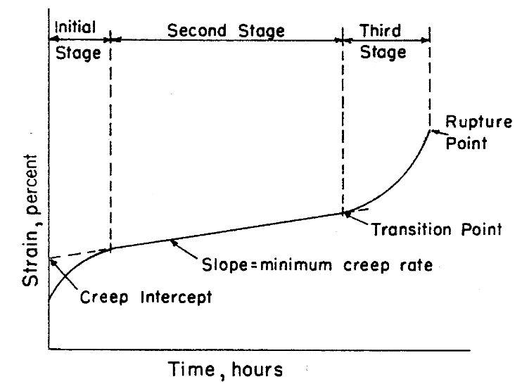
Results of creep or stress-rupture tests conducted over a range of stresses and temperatures are presented as curves of stress versus the logarithm of time to rupture. Each curve represents an average, best-fit description of measured behavior. Modification of such curves into design use are the responsibility of the design community since material applications and regulatory requirements may differ. Refer to Section 9.3.6 for data reduction and presentation methods and References 1.4.8.2.1(b) and (c).
Repeated loads are one of the major considerations for design of both commercial and military aircraft structures. Static loading, preceded by cyclic loads of lesser magnitudes, may result in mechanical behaviors lower than those published in room temperature allowables tables. A fatigue allowables development philosophy is not presented in this Handbook. However, basic laboratory test data are useful for materials selection and are provided in the appropriate materials sections.
A number of symbols and definitions are commonly used to describe fatigue test conditions, test results and data analysis techniques. The most important of these are described in Section 9.3.4.2.
In the past, common methods of obtaining and reporting fatigue data included results obtained from axial loading tests, plate bending tests, rotating bending tests, and torsion tests. Rotating bending tests apply completely reversed (tension-compression) stresses to round cross section specimens. Tests of this type are now seldom conducted for aerospace use and have therefore been dropped from importance in this Handbook. For similar reasons, flexural fatigue data also have been dropped. No significant amount of torsional fatigue data have ever been made available. Axial loading tests, the only type retained in this Handbook, consist of completely reversed loading conditions (mean stress equals zero) and those in which the mean stress was varied to create different stress (or strain) ratios (R = minimum stress or strain divided by maximum stress or strain). Refer to Reference 1.4.9(a) for load control fatigue testing guidelines and Reference 1.4.9(b) for strain control fatigue testing guidelines.
Results of axial fatigue tests are reported on S-N and ε-N diagrams. Figure 1.4.9.2(a) shows a family of axial load S-N curves. Data for each curve represents a separate R-value.
S-N and H - N diagrams are shown in this Handbook with the raw test data plotted for each stress or strain ratio or, in some cases, for a single value of mean stress. A best-fit curve is drawn through the data at each condition. Rationale used to develop best-fit curves and the characterization of all such curves in a single diagram is explained in Section 9.3.4. For load control test data, individual curves are usually based on an equivalent stress that consolidates data for all stress ratios into a single curve. Refer to Figure 1.4.9.2(b). For strain control test data, an equivalent strain consolidation method is used.
Elevated temperature fatigue test data are treated in the same manner as room temperature data, as long as creep is not a significant factor and room temperature analysis methods can be applied. In the limited number of cases where creep strain data have been recorded as a part of an elevated temperature fatigue test series, S-N (or H - N) plots are constructed for specific creep strain levels. This is provided in addition to the customary plot of maximum stress (or strain) versus cycles to failure.
The above information may not apply directly to the design of structures for several reasons. First, Handbook information may not take into account specific stress concentrations unique to any given structural design. Design considerations usually include stress concentrations caused by re-entrant corners, notches, holes, joints, rough surfaces, structural damage, and other conditions. Localized high stresses induced during the fabrication of some parts have a much greater influence on fatigue properties than on static properties. These factors significantly reduce fatigue life below that which is predictable by estimating smooth specimen fatigue performance with estimated stresses due to fabrication. Fabricated parts have been found to fail at less than 50,000 cycles of loading when the nominal stress was far below that which could be repeated many millions of times using a smooth-machined test specimen.
Notched fatigue specimen test data are shown in various Handbook figures to provide an understanding of deleterious effects relative to results for smooth specimens. All of the mean fatigue curves published in this Handbook, including both the notched fatigue and smooth specimen fatigue curves, require modification into allowables for design use. Such factors may impose a penalty on cyclic life or upon stress. This is a responsibility for the design community. Specific reductions vary between users of such information, and depending on the criticality of application, sources of uncertainty in the analysis, and requirements of the certificating activity. References 1.4.9.2(a) and (b) contain more specific information on fatigue testing procedures, organization of test results, influences of various factors, and design considerations.
. Best fit SN curve.png)
. Consolidated fatigue.png)
In addition to the retention of strength and ductility, a structural material must also retain surface and internal stability. Surface stability refers to the resistance of the material to oxidizing or corrosive environments. Lack of internal stability is generally manifested (in some ferrous and several other alloys) by carbide precipitation, spheroidization, sigma-phase formation, temper embrittlement, and internal or structural transformation, depending upon the specific conditions of exposure.
Environmental conditions, that influence metallurgical stability include heat, level of stress, oxidizing or corrosive media, and nuclear radiation. The effect of environment on the material can be observed as either improvement or deterioration of properties, depending upon the specific imposed conditions. For example, prolonged heating may progressively raise the strength of a metallic alloy as measured on smooth tensile or fatigue specimens. However, at the same time, ductility may be reduced to such an extent that notched tensile or fatigue behavior becomes erratic or unpredictable. The metallurgy of each alloy should be considered in making material selections.
Under normal temperatures, i.e., between -65°F and 160°F, the stability of most structural metallic alloys is relatively independent of exposure time. However, as temperature is increased, the metallurgical instability becomes increasingly time dependent. The factor of exposure time should be considered in design when applicable.
Discussions up to this point pertained to uniaxial conditions of static, fatigue, and creep loading. Many structural applications involve both biaxial and triaxial loadings. Because of the difficulties of testing under triaxial loading conditions, few data exist. However, considerable biaxial testing has been conducted and the following paragraphs describe how these results are presented in this Handbook. This does not conflict with data analysis methods presented in Chapter 9. Therein, statistical analysis methodology is presented solely for use in analyzing test data to establish allowables.
If stress axes are defined as being mutually perpendicular along x-, y-, and z-directions in a rectangular coordinate system, a biaxial stress is then defined as a condition in which loads are applied in both the x- and y-directions. In some special cases, loading may be applied in the z-direction instead of the y-direction. Most of the following discussion will be limited to tensile loadings in the x- and y- directions. Stresses and strains in these directions are referred to as principal stresses and principal strains. See Reference 1.4.11.
When a specimen is tested under biaxial loading conditions, it is customary to plot the results as a biaxial stress-strain diagram. These diagrams are similar to uniaxial stress-strain diagrams shown in Figure 1.4.4. Usually, only the maximum (algebraically larger) principal stress and strain are shown for each test result. When tests of the same material are conducted at different biaxial stress ratios, the resulting curves may be plotted simultaneously, producing a family of biaxial stress-strain curves as shown in Figure 1.4.11 for an isotropic material. For anisotropic materials, biaxial stress-strain curves also require distinction by grain direction.
The reference direction for a biaxial stress ratio, i.e., the direction corresponding to B=0, should be clearly indicated with each result. The reference direction is always considered as the longitudinal (rolling) direction for flat products and the hoop (circumferential) direction for shells of revolution, e.g., tubes, cones, etc. The letter B denotes the ratio of applied stresses in the two loading directions. For example, biaxility ratios of 2 and 0.5 shown in Figure 1.4.11 indicate results representing both biaxial stress ratios of 2 or 0.5, since this is a hypothetical example for an isotropic material, e.g., cross-rolled sheet. In a similar manner, the curve labeled B=1 indicates a biaxial stress-strain result for equally applied stresses in both directions. The curve labeled B = ∞, 0 indicates the biaxial stress-strain behavior when loading is applied in only one direction, e.g., uniaxial behavior. Biaxial property data presented in the Handbook are to be considered as basic material properties obtained from carefully prepared specimens.
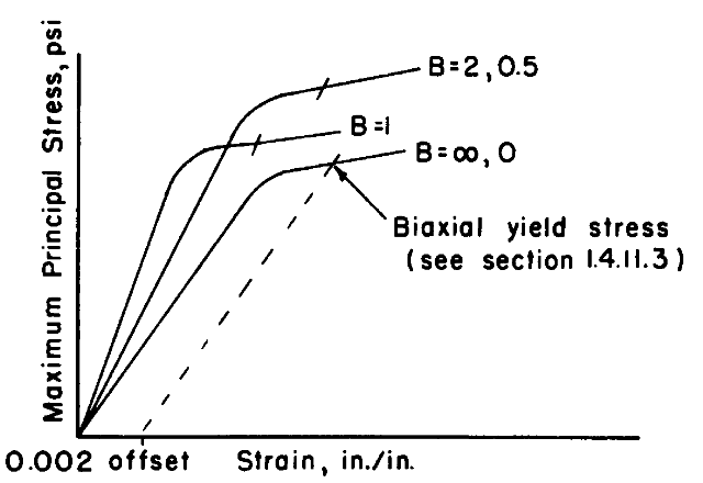
Referring to Figure 1.4.11, it is noted that the original portion of each stress-strain curve is essentially a straight line. Under biaxial loading conditions, the initial slope of such curves is defined as the biaxial modulus. It is a function of biaxial stress ratio and Poisson's ratio. See Equation 1.3.7.4.
Biaxial yield stress is defined as the maximum principal stress corresponding to 0.002 in./in. plastic strain in the same direction, as determined from a test curve.
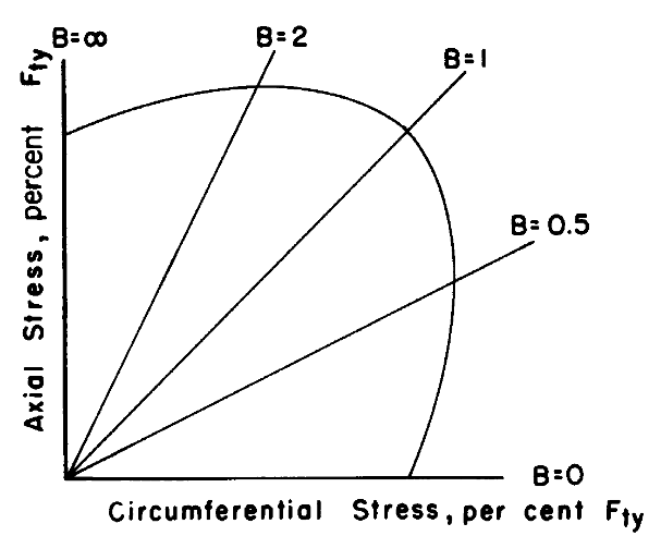
In the design of aerospace structures, biaxial stress ratios other than those normally used in biaxial testing are frequently encountered. Information can be combined into a single diagram to enable interpolations at intermediate biaxial stress ratios, as shown in Figure 1.4.11.2. An envelope is constructed through test results for each tested condition of biaxial stress ratios. In this case, a typical biaxial yield stress envelope is identified. In the preparation of such envelopes, data are first reduced to nondimensional form (percent of uniaxial tensile yield stress in the specified reference direction), then a best-fit curve is fitted through the nondimensionalized data. Biaxial yield strength allowables are then obtained by multiplying the uniaxial Fty (or Fcy) allowable by the applicable coordinate of the biaxial stress ratio curve. To avoid possible confusion, the reference direction used for the uniaxial yield strength is indicated on each figure.
Biaxial ultimate stress is defined as the highest nominal principal stress attained in specimens of a given configuration, tested at a given biaxial stress ratio. This property is highly dependent upon geometric configuration of the test parts. Therefore, such data should be limited in use to the same design configurations.
The method of presenting biaxial ultimate strength data is similar to that described in the preceding section for biaxial yield strength. Both biaxial ultimate strength and corresponding uniform elongation data are reported, when available, as a function of biaxial stress ratio test conditions
The occurrence of flaws in a structural component is an unavoidable circumstance of material processing, fabrication, or service. Flaws may appear as cracks, voids, metallurgical inclusions, weld defects, design discontinuities, or some combination thereof. The fracture toughness of a part containing a flaw is dependent upon flaw size, component geometry, and a material property defined as fracture toughness. The fracture toughness of a material is literally a measure of its resistance to fracture. As with other mechanical properties, fracture toughness is dependent upon alloy type, processing variables, product form, geometry, temperature, loading rate, and other enviro- nmental factors.
This discussion is limited to brittle fracture, which is characteristic of high strength materials under conditions of loading resulting in plane-strain through the cross section. Very thin materials are described as being under the condition of plane-stress. The following descriptions of fracture toughness properties applies to the currently recognized practice of testing specimens under slowly increasing loads. Attendant and interacting conditions of cyclic loading, prolonged static loadings, environmental influences other than temperature, and high strain rate loading are not considered.
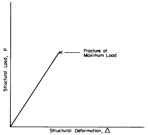
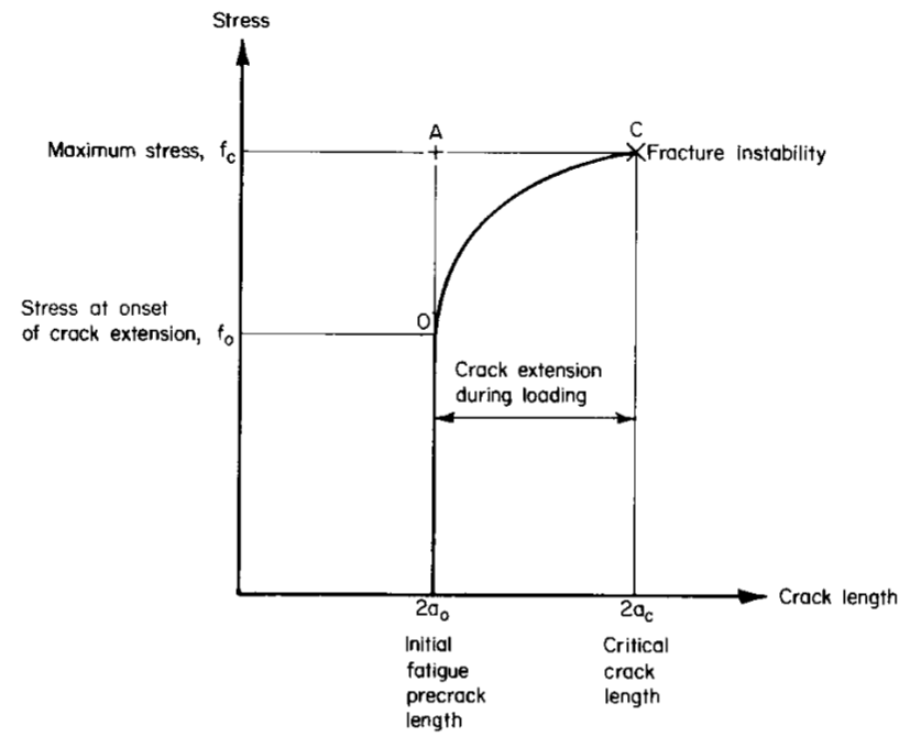
For materials that have little capacity for plastic flow, or for flaw and structural configurations, which induce triaxial tension stress states adjacent to the flaw, component behavior is essentially elastic until the fracture stress is reached. Then, a crack propagates from the flaw suddenly and completely through the component. A convenient illustration of brittle fracture is a typical load-compliance record of a brittle structural component containing a flaw, as illustrated in Figure 1.4.12.1. Since little or no plastic effects are noted, this mode is termed brittle fracture.
This mode of fracture is characteristic of the very high-strength metallic materials under plane-strain conditions.
The application of linear elastic fracture mechanics has led to the stress intensity concept to relate flaw size, component geometry, and fracture toughness. In its very general form, the stress intensity factor, K, can be expressed as:
where
f = stress applied to the gross section, ksia = measure of flaw size, inches
Y = factor relating component geometry and flaw size, nondimensional. See Reference 1.4.12.2(a) for values.
For every structural material, which exhibits brittle fracture (by nature of low ductility or plane- strain stress conditions), there is a lower limiting value of K termed the plane-strain fracture toughness, KIc.
The specific application of this relationship is dependent on flaw type, structural configuration and type of loading, and a variety of these parameters can interact in a real structure. Flaws may occur through the thickness, may be imbedded as voids or metallurgical inclusions, or may be partial-through (surface) cracks. Loadings of concern may be tension and/or flexure. Structural components may vary in section size and may be reinforced in some manner. The ASTM Committee E 8 on Fatigue and Fracture has developed testing and analytical techniques for many practical situations of flaw occurrence subject to brittle fracture. They are summarized in Reference 1.4.12.2(a).
A tabulation of fracture toughness data is printed in the general discussion prefacing most alloy chapters in this Handbook. These critical plane-strain fracture toughness values have been determined in accordance with recommended ASTM testing practices. This information is provided for information purposes only due to limitations in available data quantities and product form coverages. The statistical reliability of these properties is not known. Listed properties generally represent the average value of a series of test results.
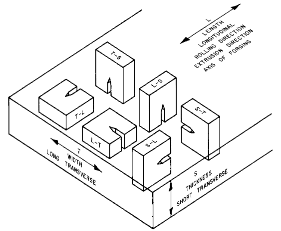
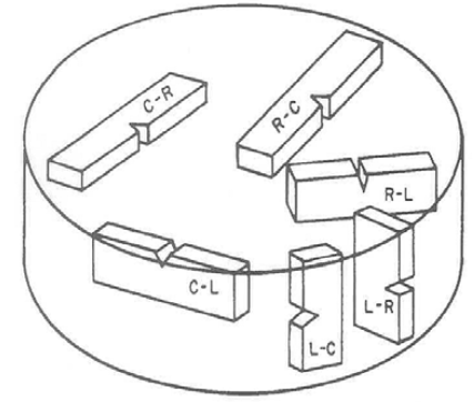
Fracture toughness of a material commonly varies with grain direction. When identifying either test results or a general critical plane strain fracture toughness average value, it is customary to specify specimen and crack orientations by an ordered pair of grain direction symbols per ASTM E399. [Reference 1.4.12.2(a).] The first digit denotes the grain direction normal to the crack plane. The second digit denotes the grain direction parallel to the fracture plane. For flat sections of various products, e.g., plate, extrusions, forgings, etc., in which the three grain directions are designated (L) longitudinal, (T) transverse, and (S) short transverse, the six principal fracture path directions are: L-T, L-S, T-L, T-S, S-L and S-T. Figure 1.4.12.3(a) identifies these orientations. For cylindrical sections where the direction of principle deformation is parallel to the longitudinal axis of the cylinder, the reference directions are identified as in Figure 1.4.12.3(b), which gives examples for a drawn bar. The same system would be useful for extrusions or forged parts having circular cross section.
Cyclic loading, even well below the fracture threshold stress, may result in the propagation of flaws, leading to fracture. Strain rates in excess of standard static rates may cause variations in fracture toughness properties. There are significant influences of temperature on fracture toughness properties. Temperature effects data are limited. These information are included in each alloy section, when available.
Under the condition of sustained loading, it has been observed that certain materials exhibit increased flaw propagation tendencies when situated in either aqueous or corrosive environments. When such is known to be the case, appropriate precautionary notes have been included with the standard fracture toughness information.
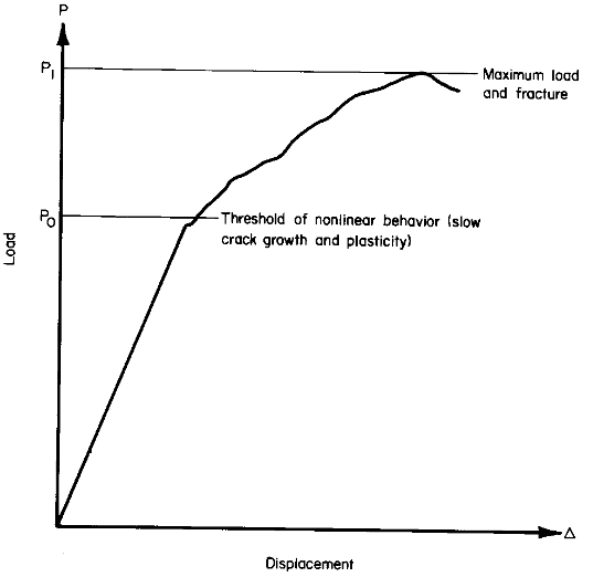
Plane-strain conditions do not describe the condition of certain structural configurations which are either relatively thin or exhibit appreciable ductility. In these cases, the actual stress state may approach the opposite extreme, plane-stress, or, more generally, some intermediate- or transitional-stress state. The behavior of flaws and cracks under these conditions is different from those of plane-strain. Specifically, under these conditions, significant plastic zones can develop ahead of the crack or flaw tip, and stable extension of the discontinuity occurs as a slow tearing process. This behavior is illustrated in a compliance record by a significant nonlinearity prior to fracture as shown in Figure 1.4.12.4. This nonlinearity results from the alleviation of stress at the crack tip by causing plastic deformation.
The basic concepts of linear elastic fracture mechanics as used in plane-strain fracture analysis also applies to these conditions. The stress intensity factor concept, as expressed in general form by Equation 1.4.12.2, is used to relate load or stress, flaw size, component geometry, and fracture toughness.
However, interpretation of the critical flaw dimension and corresponding stress has two possibilities. This is illustrated in Figure 1.4.12.4.1. One possibility is the onset of nonlinear displacement with increasing load. The other possibility identifies the fracture condition, usually very close to the maximum load. Generally, these two conditions are separated in applied stress and exhibit large differences in flaw dimensions due to stable tearing.
When a compliance record is transformed into a crack growth curve, the difference between the two possible K-factor designations becomes more apparent. In most practical cases, the definition of nonlinear crack length with increasing load is difficult to assess. As a result, an alternate characterization of this behavior is provided by defining an artificial or “apparent” stress intensity factor.
The apparent fracture toughness is computed as a function of the maximum stress and initial flaw size. This datum coordinate corresponds to point A in Figure 1.4.12.4.1. This conservative stress intensity factor is a first approximation to the actual property associated with the point of fracture.
When available, each alloy chapter contains graphical formats of stress versus flaw size. This is provided for each temper, product form, grain direction, thickness, and specimen configuration. Data points shown in these graphs represent the initial flaw size and maximum stress achieved. These data have been screened to assure that an elastic instability existed at fracture, consistent with specimen type. The average Kapp curve, as defined in the following subsections, is shown for each set of data.
The calculation of apparent fracture toughness for middle-tension panels is given by the following equation.
Data used to compute Kapp values have been screened to ensure that the net section stress at failure did not exceed 80 percent of the tensile yield strength; that is, they satisfied the criterion:
This criterion assures that the fracture was an elastic instability and that plastic effects are negligible.
The average Kapp parametric curve is presented on each figure as a solid line with multiple extensions where width effects are displayed in the data. As added information, where data are available, the propensity for slow stable tearing prior to fracture is indicated by a crack extension ratio, Δ2a/2ao. The coefficient (2) indicates the total crack length; the half-crack length is designated by the letter “a.” In some cases, where data exist covering a wide range of thicknesses, graphs of Kapp versus thickness are presented.
Crack growth deals with material behavior between crack initiation and crack instability. In small size specimens, crack initiation and specimen failure may be nearly synonymous. However, in larger structural components, the existence of a crack does not necessarily imply imminent failure. Significant structural life exists during cyclic loading and crack growth.
Fatigue crack growth is manifested as the growth or extension of a crack under cyclic loading. This process is primarily controlled by the maximum load or stress ratio. Additional factors include environment, loading frequency, temperature, and grain direction. Certain factors, such as environment and loading frequency, have interactive effects. Environment is important from a potential corrosion viewpoint. Time at stress is another important factor. Standard testing procedures are documented in Reference 1.4.13.1.
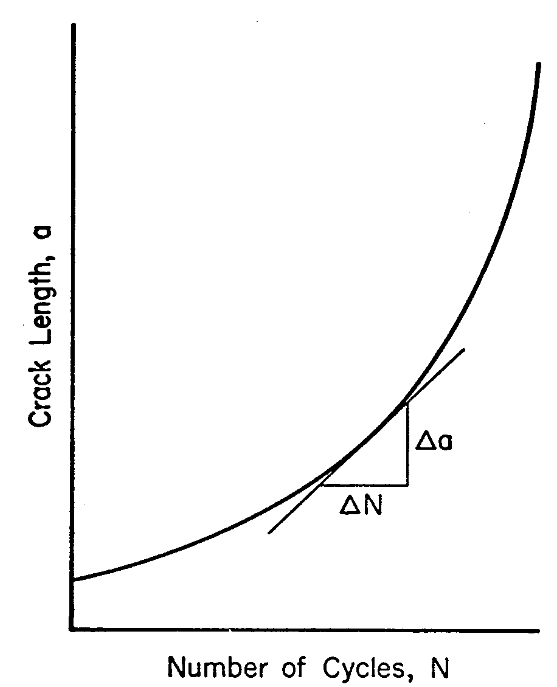
Fatigue crack growth data presented herein are based on constant amplitude tests. Crack growth behaviors based on spectrum loading cycles are beyond the scope of this Handbook. Constant amplitude data consist of crack length measurements at corresponding loading cycles. Such data are presented as crack growth curves as shown in Figure 1.4.13.1(a).
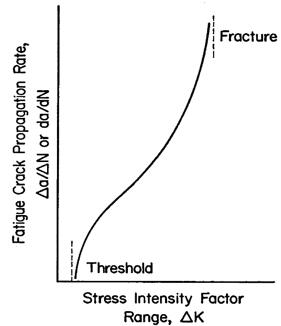
Since the crack growth curve is dependent on initial crack length and the loading conditions, the above format is not the most efficient form to present information. The instantaneous slope, Δa/ΔN, corresponding to a prescribed number of loading cycles, provides a more fundamental characterization of this behavior. In general, fatigue crack growth rate behavior is evaluated as a function of the applied stress intensity factor range, ΔK, as shown in Figure 1.4.13.1(b).
It is known that fatigue-crack-growth behavior under constant-amplitude cyclic conditions is influenced by maximum cyclic stress, Smax, and some measure of cyclic stress range, ΔS (such as stress ratio, R, or minimum cyclic stress, Smin), the instantaneous crack size, a, and other factors such as environment, frequency, and temperature. Thus, fatigue-crack-growth rate behavior can be characterized, in general form, by the relation
By applying concepts of linear elastic fracture mechanics, the stress and crack size parameters can be combined into the stress-intensity factor parameter, K, such that Equation 1.4.13.3(a) may be simplified to
where
Kmax = the maximum cyclic stress-intensity factor
ΔK = (1-R)Kmax, the range of the cyclic stress-intensity factor, for R ≥ 0
ΔK = Kmax, for R ≤ 0.
At present, in the Handbook, the independent variable is considered to be simply ǻK and the data are con- sidered to be parametric on the stress ratio, R, such that Equation 1.4.13.3(b) becomes
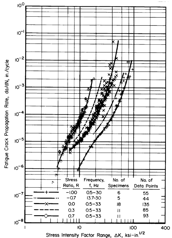
Fatigue crack growth rate data for constant amplitude cyclic loading conditions are presented as logarithmic plots of da/dN versus ǻK. Such information, such as that illustrated in Figure 1.4.13.3, are arranged by material alloy and heat treatment condition. Each curve represents a specific stress ratio, R, environment, and cyclic loading frequency. Specific details regarding test procedures and data interpolations are presented in Chapter 9.
In the following discussion, failure will usually indicate fracture of a member or the condition of a member when it has attained maximum load.
Fracture can occur in either ductile or brittle fashions in the same material depending on the state of stress, rate of loading, and environment. The ductility of a material has a significant effect on the ability of a part to withstand loading and delay fracture. Although not a specific design property for ductile materials, some ductility data are provided in the Handbook to assist in material selections. The following paragraphs discuss the relationship between failure and the applied or induced stresses.
This type of failure is associated with ultimate tensile or compressive stress of the material. For compression, it can only apply to members having large cross sectional dimensions relative to their lengths. See Section 1.4.5.1
Pure shear failures are usually obtained when the shear load is transmitted over a very short length of a member. This condition is approached in the case of rivets and bolts. In cases where ultimate shear stress is relatively low, a pure shear failure can result. But, generally members subjected to shear loads fail under the action of the resulting normal stress, usually the compressive stress. See Equation 1.3.3.3. Failure of tubes in torsion are not caused by exceeding the shear ultimate stress, but by exceeding a normal compressive stress which causes the tube to buckle. It is customary to determine stresses for members subjected to shear in the form of shear stresses although they are actually indirect measures of the stresses actually causing failure.
Failure of a material in bearing can consist of crushing, splitting, tearing, or progressive rapid yielding in the direction of load application. Failure of this type depends on the relative size and shape of the two connecting parts. The maximum bearing stress may not be applicable to cases in which one of the connecting members is relatively thin.
For sections not subject to geometric instability, a bending failure can be classed as either a tensile or compressive failure. Reference 1.5.2.4 provides methodology by which actual bending stresses above the material proportional limit can be used to establish maximum stress conditions. Actual bending stresses are related to the bending modulus of rupture. The bending modulus of rupture (fb) is determined by Equation 1.3.2.3. When the computed bending modulus of rupture is found to be lower than the proportional limit strength, it represents an actual stress. Otherwise, it represents an apparent stress, and is not considered as an actual material strength. This is important when considering complex stress states, such as combined bending and compression or tension.
Static stress properties represent pristine materials without notches, holes, or other stress concentrations. Such simplistic structural design is not always possible. Consideration should be given to the effect of stress concentrations. When available, references are cited for specific data in various chapters of the Handbook.
Under combined stress conditions, where failure is not due to buckling or instability, it is necessary to refer to some theory of failure. The “maximum shear” theory is widely accepted as a working basis in the case of isotropic ductile materials. It should be noted that this theory defines failure as the first yielding of a material. Any extension of this theory to cover conditions of final rupture must be based on evidence supported by the user. The failure of brittle materials under combined stresses is generally treated by the “maximum stress” theory. Section 1.4.11 contains a more complete discussion of biaxial behavior. References 1.5.2.6(a) through (c) offer additional information.
Practically all structural members, such as beams and columns, particularly those made from thin material, are subject to failure due to instability. In general, instability can be classed as (1) primary or (2) local. For example, the failure of a tube loaded in compression can occur either through lateral deflection of the tube acting as a column (primary instability) or by collapse of the tube walls at stresses lower than those required to produce a general column failure. Similarly, an I-beam or other formed shape can fail by a general sidewise deflection of the compression flange, by local wrinkling of thin outstanding flanges, or by torsional instability. It is necessary to consider all types of potential failures unless it is apparent that the critical load for one type is definitely the controlling condition.
Instability failures can occur in either the elastic range below the proportional limit or in the plastic range. These two conditions are distinguished by referring to either “elastic instability” or “plastic instability” failures. Neither type of failure is associated with a material’s ultimate strength, but largely depends upon geometry.
A method for determining the local stability of aluminum alloy column sections is provided in Reference 1.7.1(b). Documents cited therein are the same as those listed in References 3.20.2.2(a) through (e).
Failures of this type are discussed in Section 1.6 (Columns).
Round tubes when subjected to bending are subject to plastic instability failures. In such cases, the failure criterion is the modulus of rupture. Equation 1.3.2.3, which was derived from theory and confirmed empirically with test data, is applicable. Elastic instability failures of thin walled tubes having high D/t ratios are treated in later sections.
The remarks given in the preceding section apply in a similar manner to round tubes under torsional loading. In such cases, the modulus of rupture in torsion is derived through the use of Equation 1.3.2.6. See Reference 1.5.3.3.
For combined loading conditions in which failure is caused by buckling or instability, no theory exists for general application. Due to the various design philosophies and analytical techniques used throughout the aerospace industry, methods for computing margin of safety are not within the scope of this Handbook.
A theoretical treatment of columns can be found in standard texts on the strength of materials. Some of the problems which are not well defined by theory are discussed in this section. Actual strengths of columns of various materials are provided in subsequent chapters.
A column can fail through primary instability by bending laterally (stable sections) or by twisting about some axis parallel to its own axis. This latter type of primary failure is particularly common to columns having unsymmetrical open sections. The twisting failure of a closed section column is precluded by its inherently high torsional rigidity. Since the amount of available information is limited, it is advisable to conduct tests on all columns subject to this type of failure.
The Euler formula for columns which fail by lateral bending is given by Equation 1.3.8.2. A conservative approach in using this equation is to replace the elastic modulus (E) by the tangent modulus (Et) given by Equation 1.3.8.1. Values for the restraint coefficient (c) depend on degrees of ends and lateral fixities. End fixities tend to modify the effective column length as indicated in Equation 1.3.8.1. For a pin-ended column having no end restraint, c = 1.0 and L1 = L. A fixity coefficient of c = 2 corresponds to an effective column length of L1 = 0.707 times the total length.
The tangent modulus equation takes into account plasticity of a material and is valid when the following conditions are met:
- he column adjusts itself to forcible shortening only by bending and not by twisting.
- No buckling of any portion of the cross section occurs.
- Loading is applied concentrically along the longitudinal axis of the column.
- The cross section of the column is constant along its entire length.
MIL-HDBK-5 provides typical stress versus tangent modulus diagrams for many materials, forms, and grain directions. These information are not intended for design purposes. Methodology is contained in Chapter 9 for the development of allowable tangent modulus curves.
The upper limit of column stress for primary failure is designated as fco. By definition, this term should not exceed the compression ultimate strength, regardless of how the latter term is defined.
Methods of analysis by which column failure stresses can be computed, accounting for fixities, torsional instability, load eccentricity, combined lateral loads, or varying column sections are contained in References 1.6.2.3(a) through (d).
Columns are subject to failure by local collapse of walls at stresses below the primary failure strength. The buckling analysis of a column subject to local instability requires consideration of the shape of the column cross section and can be quite complex. Local buckling, which can combine with primary buckling, leads to an instability failure commonly identified as crippling.
The upper limit of column stress for local failure is defined by either its crushing or crippling stress. The strengths of round tubes have been thoroughly investigated and considerable amounts of test results are available throughout literature. Fewer data are available for other cross sectional configurations and testing is suggested to establish specific information, e.g., the curve of transition from local to primary failure.
In the case of columns having unconventional cross sections which are subject to local instability, it is necessary to establish curves of transition from local to primary failure. In determining these column curves, sufficient tests should be made to cover the following points.
Test specimens should cover a range of L'/ρ values. When columns are to be attached eccentrically in structural application, tests should be designed to cover such conditions. This is important particularly in the case of open sections, as maximum load carrying capabilities are affected by locations of load and reaction points.
When local failure occurs, the crushing or crippling stress can be determined by extending the short column curve to a point corresponding to a zero value for L'/ρ'. When a family of columns of the same general cross section is used, it is often possible to determine a relationship between crushing or crippling stress and some geometric factor. Examples are wall thickness, width, diameter, or some combination of these dimensions. Extrapolation of such data to conditions beyond test geometry extremes should be avoided.
The use of correction factors provided in Figures 1.6.4.3(a) through (i) is acceptable to the Air Force, the Navy, the Army, and the Federal Aviation Administration for use in reducing aluminum and magnesium alloys column test data into allowables. (Note that an alternate method is provided in Section 1.6.4.4). In using Figures 1.6.4.3(a) through (i), the correction of column test results to standard material is made by multiplying the stress obtained from testing a column specimen by the factor K. This factor may be considered applicable regardless of the type of failure involved, i.e., column crushing, crippling or twisting. Note that not all the information provided in these figures pertains to allowable stresses, as explained below.
The following terms are used in reducing column test results into allowable column stress:
Fcy is the design compression yield stress of the material in question, applicable to the gage, temper and grain direction along the longitudinal axis of a test column.
Fc' is the maximum test column stress achieved in test. Note that a letter °F) is used rather the customary lower case (f). This value can be an individual test result.
Fcy' is the compressive yield strength of the column material. Note that a letter °F) is used rather than the customary lower case (f). This value can be an individual test result using a standard compression test specimen.
Using the ratio of (Fc' / Fcy'), enter the appropriate diagram along the abscissa and extend a line upwards to the intersection of a curve with a value of (Fc' / Fcy'). Linear interpolation between curves is permissible. At this location, extend a horizontal line to the ordinate and read the corresponding K-factor. This factor is then used as a multiplier on the measured column strength to obtain the allowable. The basis for this allowable is the same as that noted for the compression yield stress allowable obtained from the room temperature allowables table.
If the above method is not feasible, due to an inability of conducting a standard compression test of the column material, the compression yield stress of the column material may be estimated as follows: Conduct a standard tensile test of the column material and obtain its tensile yield stress. Multiply this value by the ratio of compression-to-tensile yield allowables for the standard material. This provides the estimated compression yield stress of the column material. Continue with the analysis as described above using the compression stress of a test column in the same manner.
If neither of the above methods are feasible, it may be assumed that the compressive yield stress allowable for the column is 15 percent greater than minimum established allowable longitudinal tensile yield stress for the material in question.
For materials that are not covered by Figures 1.6.4.4(a) through (i), the following method is acceptable for all materials to the Air Force, the Navy, the Army, and the Federal Aviation Administration.
(1) Obtain the column material compression properties: Fcy, Ec, nc.
(2) Determine the test material column stress (fc') from one or more column tests
(3) Determine the test material compression yield stress (fcy'') from one or more tests.
(4) Assume Ec and nc from (1) apply directly to the column material. They should be the same material.
(5) Assume that geometry of the test column is the same as that intended for design. This means that a critical slenderness ratio value of (L'/ρ) applies to both cases.
(6) Using the conservative form of the basic column formula provided in Equation 1.3.8.1, this enables an equality to be written between column test properties and allowables. If
(L'/ρ) for design = (L'/ρ) of the column test
Then
(Fc/Et) for design = (Fc'/Et') from test
(7) Tangent modulus is defined as:
(8) Total strain (e) is defined as the sum of elastic and plastic strains, and throughout the Handbook is used as:
or,
. Nondimensional material.png)
. Nondimensional material correction.png)
.png)
.png)
.png)
.png)
.png)
.png)
.png)
Equation 1.6.4.4(c) can be rewritten as follows:
Tangent modulus, for the material in question, using its compression allowables is:
In like manner, tangent modulus for the same material with the desired column configuration is:
Substitution of Equations 1.6.4.4(g) and 1.6.4.4(h) for their respective terms in Equation 1.6.4.4(b) and simplifying provides the following relationship:
The only unknown in the above equation is the term Fc, the allowable column compression stress. This property can be solved by an iterative process.
This method is also applicable at other than room temperature, having made adjustments for the effect of temperature on each of the properties. It is critical that the test material be the same in all respects as that for which allowables are selected from the Handbook. Otherwise, the assumption made in Equation 1.6.4.4(c) above is not valid. Equation 1.6.4.4(i) must account for such differences in moduli and shape factors when applicable.
A bibliography of information on thin-walled and stiffened thin-walled sections is contained in References 1.7(a) and (b).