NSWC-11 Shaft Reliability Model

A shaft is a rotating member, usually round, that carries power or motion and holds gears, pulleys, impellers and couplings on its axis. It is normally designed for an infinite life, so the shaft itself rarely fails. Studies cited in the handbook put its failure rate at about one eighth of a mechanical seal and one third of a ball bearing. Where a shaft does matter is in what it does to its neighbors. Excess bending misaligns gears and wears bearings and seals.

This tool follows Chapter 20 of the Naval Surface Warfare Center Handbook of Reliability Prediction Procedures for Mechanical Equipment (NSWC-11). The base failure rate comes from the number of cycles to failure at the stress the shaft sees. It is then multiplied by factors for surface finish, temperature, shaft displacement and stress concentration at shoulders and grooves. It also gives the torque and shear stress from the handbook’s Eq. 20-1 and 20-2.

The result is a failure rate per million cycles and per million hours, with FIT and MTBF for a FMECA. Every step of the working is under “Show detailed calculation steps”. A shaft failure rate is usually added to the rates of the pump, motor or compressor it belongs to.
NSWC-11 Chapter 20 Failure Rate Calculator
Shaft Reliability (NSWC-11 Eq. 20-3)
Material & Endurance Limit
Steel up to 200 ksi: 0.5 Tult. Steel above 200 ksi: 100 ksi. Other metals use the Table 20-2 ratios.
Cycles to Failure & Speed
The handbook sets the base rate to 1/N, where N is the number of cycles to failure at the stress the shaft sees.
The handbook uses 108 cycles for materials with no definite endurance limit.
1 for a rotating shaft in fixed-direction bending. Use 2 or more where the load reverses more than once per turn.
Torque & Shear Stress (information)
Used with the speed above to give the torque (Eq. 20-1). Set to 0 to skip.
The diameter at the section you want the torsional shear stress for (Eq. 20-2).
Surface Finish & Temperature
The factor also uses the tensile strength above.
The Table 20-3 values fall for rougher finishes, which lowers the rate. See the surface finish card.
The factor starts above 160 °F (71 °C).
Shaft Displacement (CDY)
Sets the allowable shaft deflection b.
Fluid radial unbalance force or load weight acting on the shaft.
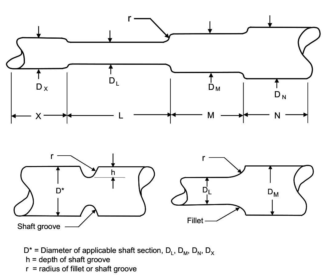
Shaft Sections (Figure 20.2)
Up to four sections, X, L, M and N, left to right. Leave a length at 0 to drop that section.
Stress Concentration (CSC)
Shoulder Fillet (Eq. 20-10)
The handbook calls D the initial diameter and d the transitioned one. The equation only gives a factor above 1 when D is the larger.
Mission (optional)
8,760 h is one year of continuous operation. Leave blank to skip.
Failure Rate & Reliability Metrics
Predicted Failure Rate, λ (failures / 106 h) iλSH = λSH,B × Cf × CT × CDY × CSC, in failures per 106 cycles, then multiplied by the cycles per hour to give failures per 106 hours.
–
Failure Rate (FIT) iFailures In Time = failures per 109 hours. The same number as failures per million hours, multiplied by 1000.
–
MTBF (hours) iMean time between failures = 106 / λ. A shaft is designed for a very long life, so this is usually large. It assumes a constant failure rate.
–
MTBF (years) iMTBF in hours divided by 24 × 365.25.
–
Expected Failures over the Mission iλ × mission hours / 106. The expected count of failures for one unit, so a value above 1 means one failure is more likely than not.
–
Survival Probability over the Mission iR(t) = e−λt, the chance one unit survives the mission with no failure, assuming a constant failure rate.
–
Intermediates
–
–
–
–
–
–
Multiplying Factors
SymbolMeaningValue
Show detailed calculation steps
How the Model Works

Shafts are designed for infinite life. So NSWC-11 treats the shaft’s failure rate as a fatigue rate set by its material. It then adjusts that rate for the conditions that make a particular shaft worse or better than the reference.

1. The equation

\[ \lambda_{SH} = \lambda_{SH,B}\cdot C_f\cdot C_T\cdot C_{DY}\cdot C_{SC} \qquad\text{(Eq. 20-3)} \]
SymbolMeaning
λSHShaft failure rate, failures per million cycles
λSH,BBase failure rate, 1/N, from the cycles to failure at the applied stress
CfSurface finish factor (Table 20-3)
CTMaterial temperature factor (Eq. 20-5)
CDYShaft displacement factor (Eq. 20-8)
CSCStress concentration factor for shoulders and grooves (Eq. 20-9)

2. What the model assumes

The equation assumes a constant rotational torque from the transmitted power and completely reversed bending from rotation. One revolution is one stress cycle. Some loading is very different, such as the large reciprocating loads in piston engines and compressors. The handbook says to analyze those cases and adjust the failure rate.

3. Units: cycles and hours

The shaft rate is per million cycles. The calculator turns it into a time rate by multiplying by the cycles per hour. That is 60 × rpm × cycles per revolution. So failures per 106 hours = (failures per 106 cycles) × cycles per hour.

4. Step by step

  1. Choose the material. The calculator looks up the endurance limit from Table 20-2 and the modulus from Table 20-5.
  2. Enter N, the cycles to failure at the applied stress, or let the page estimate it from the stress.
  3. Take 1/N as the base rate, then multiply by Cf, CT, CDY and CSC.
  4. Multiply by the cycles per hour to get a time rate. Convert to FIT and MTBF, and, with a mission time, to expected failures and survival probability.
Three places the handbook needs interpretation. The surface finish factors fall for rougher finishes, which lowers the rate (see the card). The shoulder equation is only meaningful with D as the larger diameter. And the cycles to failure N comes from an S-N curve the handbook does not supply. The page states what it does in each case and offers a switch where one is possible.
Factor Reference Guide
NSWC-11 Chapter 20: Shafts
λB

Base Failure Rate & Endurance Limit

Equations 20-4, Table 20-2
Eq. 20-4 \[ \lambda_{SH,B} = \frac{1}{N}\ \ \text{per }10^6\text{ cycles} \]

N is in millions of cycles at the stress SED.

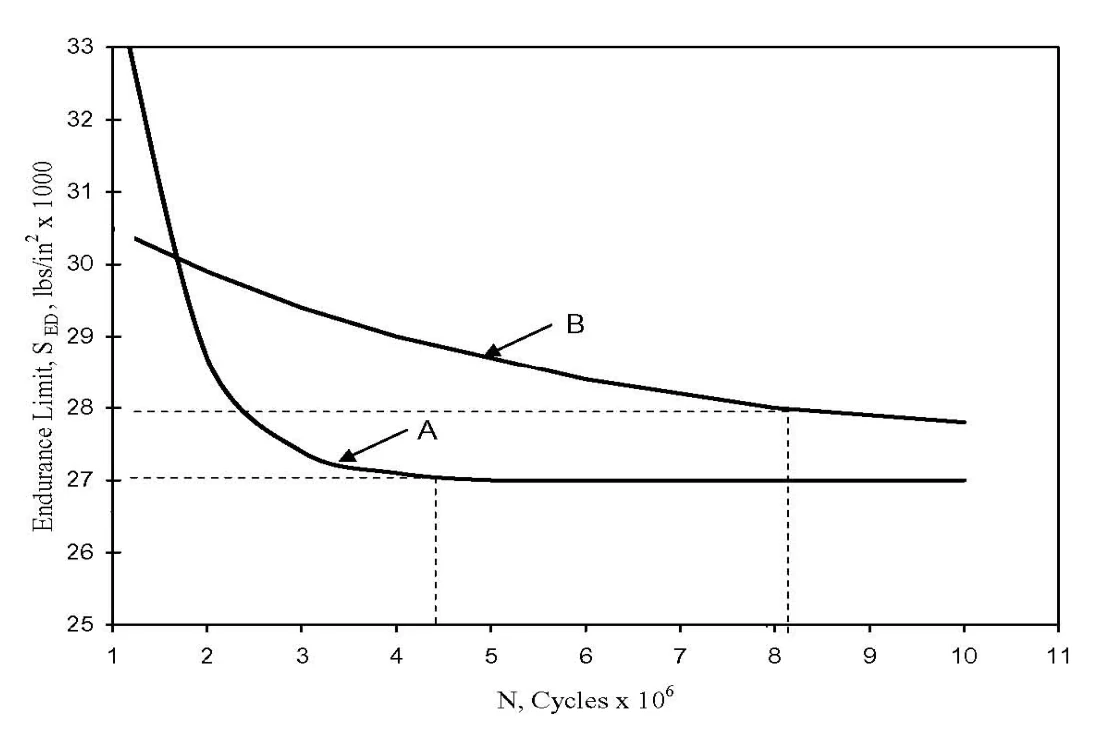
In a fatigue test a specimen is stressed to a level and the cycles to fracture are counted. Plotted, that is the S-N curve. Many ferrous metals show a flat endurance limit beyond about a million cycles (curve A of Figure 20.1). Many other materials show no definite limit, and a value is read at a chosen cycle count, usually 108 (curve B). The base failure rate is the reciprocal of the cycles to failure.

The handbook does not publish S-N curves, only the average endurance limits in Table 20-2, so N is an input. The calculator’s default is 108 cycles.

Check yourself. Figure 20.1 curve A reaches its limit at about 4.4 million cycles, so λB = 1/4.4 = 0.227 per million cycles. At 108 cycles it is 0.01 per million cycles.
Mind the time scale. 108 cycles is 926 hours at 1,800 rpm. A shaft that is well under its endurance limit lasts far longer, and a bigger N is justified there. The default sets a conservative floor.
Table 20-2: Average Endurance Limits
MaterialEndurance limit SED
Steel, Tult ≤ 200 ksi0.50 Tult
Steel, Tult > 200 ksi100 ksi
Magnesium0.35 Tult
Nonferrous alloy0.35 Tult
Aluminum alloy (wrought)0.40 Tult
Aluminum alloy (cast)0.30 Tult
Handbook reference 39 (Shigley and Mischke).
Optional: estimate N from the stress

If you know the alternating stress Sa but not N, the page can estimate it. This is an addition, not part of NSWC-11. It is a straight line on log-log axes from (103 cycles, 0.9 Tult) to (106 cycles, SED). At or below SED it uses a run-out of 108 cycles. It is the usual textbook S-N approximation. Treat the result as an estimate.

Cf

Surface Finish Factor: Cf

Table 20-3
Table 20-3
FinishCf (TS in ksi)
Polished1.0
Ground0.89
Hot rolled0.94 − 0.0046 TS + 8.37×10⁻⁶ TS2
Machined or cold drawn1.07 − 0.0051 TS + 2.21×10⁻⁵ TS2 − 3.57×10⁻⁸ TS3
Forged0.75 − 4.06×10⁻³ TS + 7.58×10⁻⁶ TS2

The factor adjusts the base rate for how the surface was made. A shaft finished differently from the design drawing changes the reliability. The polynomials are functions of the material’s tensile strength TS in ksi, because rough surfaces cost more fatigue strength in stronger steels.

Direction of the factor. These values match the familiar fatigue-strength surface factors. Those are 1.0 for a polished surface and fall for rougher ones, because a rough surface lowers fatigue strength. Used as a failure-rate multiplier as printed, a rougher finish would give a smaller rate. The page follows the handbook as printed by default and offers “Inverted (1/Cf)” if you want a rougher finish to raise the rate. Check which your analysis needs.
Cf vs tensile strength (Table 20-3)
Hot rolled, machined or cold drawn, and forged curves. Polished is 1.0 and ground is 0.89.
CT

Temperature Factor: CT

Equation 20-5
Eq. 20-5 \[ C_T = \begin{cases} 1.0 & T_{AT} \le 160\,^\circ\text{F} \\[4pt] \dfrac{460 + T_{AT}}{620} & T_{AT} > 160\,^\circ\text{F} \end{cases} \]

Typical fatigue data are taken at 160 °F. Above that, strength and creep resistance fall and thermal expansion changes the fits, so the factor rises with absolute temperature. It is the same expression the gear chapter uses. TAT is the operating temperature in °F. The page converts °C for you.

CT vs operating temperature (Eq. 20-5)
CDY

Shaft Displacement Factor: CDY

Equations 20-7 and 20-8, Table 20-6
Eq. 20-7 \[ Y = \frac{F\,l^{3}}{3\,E\,I},\qquad I = \frac{\pi d^{4}}{64} \]
Eq. 20-8 \[ C_{DY} = \frac{0.0043\,F}{E\,b}\left[\frac{X^3}{I_X} + \frac{L^3}{I_L} + \frac{M^3}{I_M} + \frac{N^3}{I_N}\right] \]

Shaft misalignment and excessive deflection hurt the bearings and seals on the shaft, and the handbook folds that into the failure rate. Eq. 20-7 is the plain deflection of an overhung load. F is the unbalance force or load weight and l is the overhang from the bearing. E is the modulus and I is the moment of inertia. Eq. 20-8 is the factor for a stepped shaft of up to four sections (Figure 20.2). Each section has its own length and diameter. b is the deflection the application allows.

The factor is dimensionless: F/(E·b) has units of 1/in2, and the bracket has units of in2. A factor below 1 means the deflection is smaller than the allowance.

Table 20-6: Allowable shaft deflection
Applicationb (in)
Actuator0.007
Compressor0.025
Motor0.010
Pump0.007
Default 0.007 in. Adjust b if your application requires or permits a different allowable bending.
Table 20-5: Shaft material strengths
MaterialTult (ksi)Endurance (ksi)σe/σuE (Mpsi)
Alloy steel100 – 24044 – 1060.4430
Stainless steel80 – 23024 – 690.3029
High carbon steel90 – 21039 – 900.4330
Cast steel, carbon70 – 10035 – 500.5030
Low alloy cast steel70 – 20035 – 1000.5030
Cast aluminum20 – 488 – 180.3810.3
Wrought aluminum22 – 838 – 290.3510.0 – 10.6
The calculator uses the Table 20-2 endurance rule (section 20.4.1 points to it). The ratios in this table are typical, and differ a little from Table 20-2 for some steels.
CSC

Stress Concentration Factor: CSC

Equations 20-9 and 20-10, Table 20-4
Eq. 20-9, 20-10 \[ C_{SC} = C_{SC,R} + C_{SC,G} \] \[ C_{SC,R} = \left(\frac{0.3}{r/d}\right)^{0.2}\left(\frac{D}{d}\right)^{1 - r/d} \]

Most shaft failures start at a change of geometry. CSC,R is the shoulder-fillet term, with r the fillet radius and D and d the two diameters. CSC,G is the groove term from Table 20-4, a function of the groove depth h, the shaft diameter D and the groove radius r. With no groove, the handbook sets CSC,G = 1.0. The two are added, so a shaft with a fillet and no groove has CSC = CSC,R + 1.

Large radii between sections lower the factor, and keyways and sharp shoulders raise it.

Which diameter is D? The handbook calls D the “initial” and d the “transitioned” diameter, with DL and DM of Figure 20.2 as examples. Worked either way, the equation gives a factor above 1 only when D is the larger diameter. With D = 1.5, d = 1.0 and r = 0.1 it gives 1.79. Swapped, it gives 0.92. The page takes D as the larger diameter and d as the smaller. If the critical section has no shoulder, the page uses 1.0 for CSC,R, which is an assumption.
Table 20-4: CSC,G for shaft grooves
h/Dh/r = 0.10.51.02.04.06.08.0
0.051.101.451.602.002.05––
0.101.001.271.401.702.002.25–
0.201.001.101.201.311.601.752.00
0.301.001.101.101.201.351.481.55
The calculator interpolates linearly between entries and holds the nearest value, with a warning, outside the table or in the blank cells.
CSC,G vs h/r (Table 20-4)
CSC,R vs r/d (Eq. 20-10)
T · SS

Torque & Shear Stress

Equations 20-1 and 20-2
Eq. 20-1, 20-2 \[ T = \frac{3.96\times10^{5}\,hp}{2\pi\,N},\qquad S_S = \frac{16\,T}{\pi\,d^{3}} \]

Shafts are primarily designed on the torsional moment they transmit. T is the torque in lb·in for a power hp (horsepower) at N rpm. SS is the torsional shear stress in psi for a solid round shaft of diameter d (in). 3.96×10⁵/(2π) = 63,025, the familiar constant. These two results are for information. They are not inputs to the failure-rate equation, which works from N.

Check yourself. 50 hp at 1,800 rpm gives T = 1,751 lb·in. In a 1.25 in shaft that is SS = 4,565 psi.
Figure 20.2: Typical shaft assembly
Figure 20.2: Typical shaft assembly with sections X, L, M and N, a groove and a fillet.
Sections X, L, M and N and their diameters feed Eq. 20-8. r and h are used by the fillet and groove terms.
F 20.1

Typical S-N Curves & Endurance Limits

Figure 20.1: Typical S-N curves and endurance limits. Curve A reaches 27,000 psi at about 4.4 million cycles; curve B reaches 28,000 psi at about 8.1 million cycles.
Handbook Figure 20.1. Curve A (mild steel) has a definite endurance limit of 27,000 psi, reached at about 4.4 million cycles. Curve B has no definite limit, and a value is read at a chosen number of cycles. An illustration from the handbook, not a design curve.
T 20-1

Shaft Failure Modes

Most shafts see combined rotational and bending stress, whether static, variable or dynamic. Keyways reduce load capacity, especially under impact or stress reversal, and changes in shaft radius concentrate stress. Large radii between sections help. Shafts in rotation can also become unstable at certain speeds. This is the critical speed, and it can destroy the shaft and damage the machine around it.

Failure modeFailure causeFailure effect
Bent shaft; excessive shaft deflection; shaft misalignmentExcessive load or torque; impact loads; bearing failure; dynamic loading; reversing loads; critical shaft speed exceeded; unbalanced loadAssembly vibration; damaged bearing, impeller, wear ring, mechanical seal or gear box; eventual shaft damage
Damaged surface finish; fretting corrosionImproper assembly; worn bearings; excessive load; corrosion; contaminants; manufacturing process; relative movement of tightly fitted partsDamaged bearing, impeller, wear ring, mechanical seal, gear box; bearing, gear or coupling corrosion
Shaft fatigue / fractureThermal expansion at high temperatures; stress riser at fillet; stress concentration at keyway; shaft radii changes; bending fatigue; excessive velocity; high torque loadSurface cracks, eventual shaft failure; shaft bearing failure
Condensed from handbook Table 20-1. The original table lists the causes and effects against merged cells, so they are grouped by mode here.
Worked Example

A pump shaft of alloy steel (Tult = 150 ksi) turns at 1,800 rpm and carries 50 hp. It is machined, runs at 200 °F, and has a 40 lb hydraulic unbalance force. Section X is 3 in of 1.25 in diameter and section L is 5 in of 1.5 in diameter. The critical section is a shoulder from 1.0 in to 1.5 in with a 0.1 in fillet, and has no groove. N is taken as 108 cycles. These are the calculator’s default inputs.

Step-by-step
  • T = 3.96×105 × 50 / (2π × 1800) = 1,751 lb·in, and SS = 16 × 1751 / (π × 1.253) = 4,565 psi
  • SED = 0.5 × 150 = 75 ksi (Table 20-2)
  • λSH,B = 1/N = 106 / 108 = 0.01 per 106 cycles
  • Cf = 1.07 − 0.0051(150) + 2.21×10⁻⁵(150)2 − 3.57×10⁻⁸(150)3 = 0.6818 (machined)
  • CT = (460 + 200)/620 = 1.0645
  • CDY = 0.0043 × 40 / (30×106 × 0.007) × [33/0.1198 + 53/0.2485] = 5.97×10⁻⁴
  • CSC,R = (0.3/0.1)0.2 × 1.50.9 = 1.7943, CSC,G = 1.0, so CSC = 2.7943

λSH = 0.01 × 0.6818 × 1.0645 × 5.97×10−4 × 2.7943 = 1.21×10⁻⁵ per 106 cycles. At 60 × 1800 = 108,000 cycles per hour that is 1.31 failures / 106 h, an MTBF of about 765,000 h (87 years). Over a year of running the expected failure count is 0.011 and the survival probability is 98.9 %.

The shaft rate is small next to the bearing and gear examples. That fits the handbook’s remark that the shaft itself is seldom the first thing to fail. Most of the rate comes from the stress concentration (2.79) and from the 108-cycle base rate. Try adding a groove with h = 0.1, D = 1 and r = 0.1. That gives CSC,G = 1.40, and the rate rises by about 14 %.

Important Notices
  • Not an official DoD document. NSWC-11 is the product of a Naval Surface Warfare Center research program, approved for public release. The handbook cautions that limited funding prevented full validation of every prediction equation. It should not be treated as an official Department of Defense standard.
  • No Navy affiliation or endorsement. The Naval Surface Warfare Center, Carderock Division and the U.S. Navy have not participated in the development of this calculator and do not approve or endorse it.
  • Use with the full procedure. NSWC-11 warns against extracting equations without regard to application procedures and parameter limits. Results are a design screening tool, not a substitute for the manufacturer’s rating, testing, or the judgment of a qualified engineer.
  • Shaft only. The shaft rate is for the shaft itself. The bearings, seals, couplings and gears on it have their own rates. The handbook says to add the shaft rate to those of the pump, motor or compressor it belongs to.
  • N is an input. The handbook gives no S-N curves, so the cycles to failure N must come from your material data. The optional estimate on the page is an addition and is not part of NSWC-11.
  • Interpretations. Three points are read as the cards describe. They are the direction of the surface factor, D as the larger diameter in the shoulder equation, and the neutral value 1.0 for a missing shoulder.
  • Critical speed is not modeled. The model covers fatigue, finish, temperature, deflection and stress concentration. It does not check the shaft’s critical speed, which is a separate failure mode in Table 20-1.

Cite This Work